Bruker AVANCE NEO User Guide

Introductory Theory and Terminology
H171804E_14_001 11 / 86
Note that there are experiments in which more than one nucleus gets excited, e.g. during
polarization transfer or decoupling. In these cases one has more than one carrier frequency
but still only one observe frequency.
Not all isotopes will respond to radio frequency pulses, i.e. not all are NMR active. Three
isotopes of the element hydrogen are found in nature:
1
H (hydrogen),
2
H (deuterium), and
3
H
(tritium, radioactive!). The natural abundance of these isotopes are 99.98%, 0.015%, and
0.005% respectively. All three are NMR active, although as can be seen in table 3.1, they all
display a large variation in resonance frequency. To analyze a sample for hydrogen, the
1
H
isotope is excited, as this isotope is by far the most abundant. Of the carbon isotopes found
in nature, only one is NMR active. By far the most common isotope,
12
C (98.89% natural
abundance) is inactive. Hence, NMR analysis of organic compounds for carbon rely on the
signals emitted by the
13
C isotope, which has a natural abundance of only 1.11%. Obviously,
NMR analysis for carbon is more difficult than that of, for example,
1
H (there are other factors
which affect sensitivity, these will be discussed in the next sections of this chapter).
Using the brief introduction to NMR outlined above, it is a good exercise to consider how the
technique could be used to analyze the composition of chloroform (CHCl
3
).
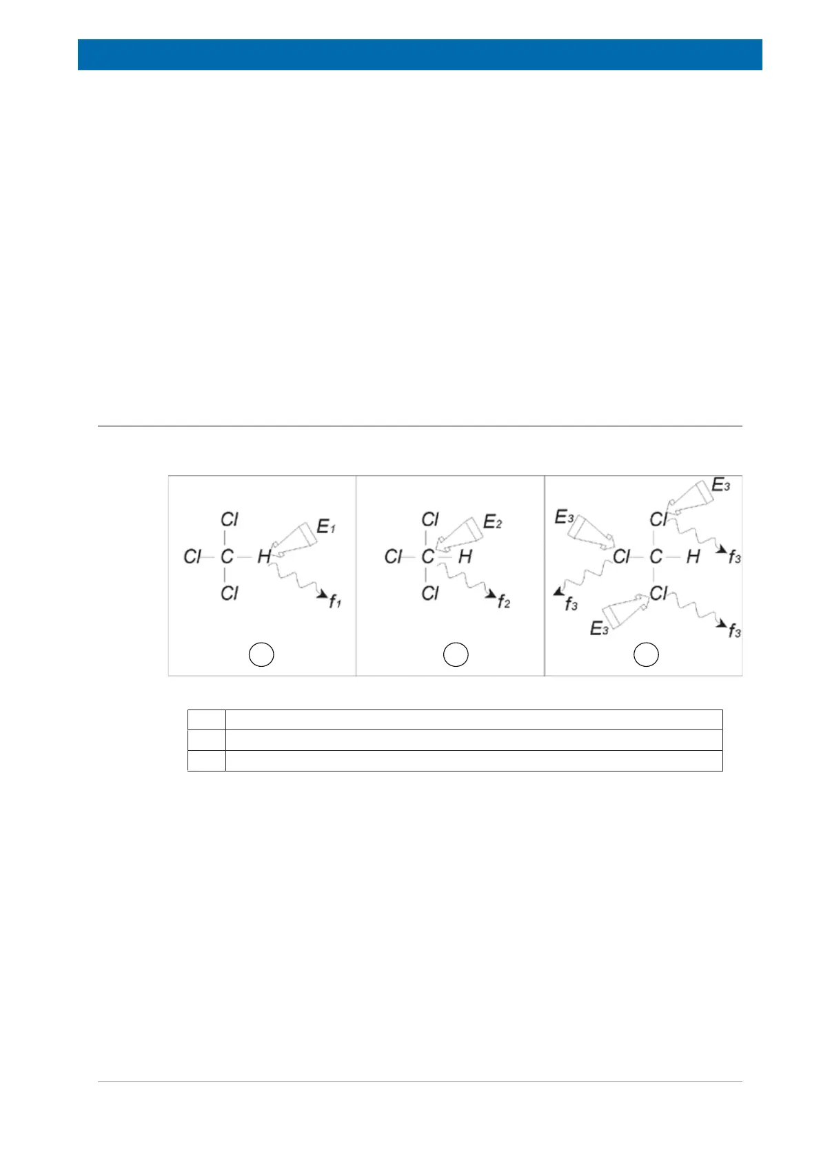
3.1 NMR Analysis of Chloroform
Three separate experiments, as outlined in the figure below, can be performed corresponding
to the three possible observe nuclei
1
H,
13
C and
35
Cl.
1 2 3
Figure3.3: NMR Analysis of CHCI3
1 Excitation E
1
2 Excitation E
2
3 Excitation E
3
Three excitation pulses (E
1
, E
2
, E
3
) are directed at the sample at appropriate carrier
frequencies. E
1
corresponds to the
1
H resonance frequency, E
2
to the
13
C frequency, and E
3
to the
35
Cl frequency. Assuming the three isotopes were successfully excited, the sample will
emit signals at three frequencies f
1
, f
2
and f
3
which are recorded on three separate spectra. If
the emitted signals are displayed in a single plot, the user can expect a spectrum like that in
the figure below (note that the signal frequencies illustrated are for a 11.7 T magnet and that
all signals have been plotted as singlets, i.e. single peaks).

Bruker AVANCE NEO Specifications

General

Brand	Bruker
Model	AVANCE NEO
Category	Laboratory Equipment
Language	English