Solartron 1260 - Page 83

Table
5.1 Measurement
Source
and
Displayed
Coordinates
SOURCE
-^COORDS
[Zl
=
Vl/I]
Yl
=
I/Vl
Z2
—
V2/
I
Y2
=
I/V2
FUNCTION
( )
VI
V2
V1./V2
V2/V1
I
Z,0
[L(orC),R] L(orC),Q L(orC),D
R,X
Y,
0 [L(orC),R] L(orC),Q L(orC),D
G,B
Z,
0
[L(orC),R]
L(orC),Q L(orC),D R,X
Y,0
[L(orC),R] L(orC),Q L(orC),D
G,B
[r,0]
r(dB),0
r,t* r(dB),t*
L(orC),R L(orC),Q L(orC),D
a,b
r,0
[r(dB),0]
r,t
r(dB),t
a,b
r,0
[r(dB),0]
r,t r(dB),t
a,b
r,0 [r(dB),0]
r,t r(dB),t
a,b
r,0
[r(dB),0]
r,t r(dB),t
a,b
[r,0]
a,b
*
For time scale measurements
use the
analyser 'group delay' mode.
(See Section 2.1.4.)
4.1.3 PHASE
Phase presentation:
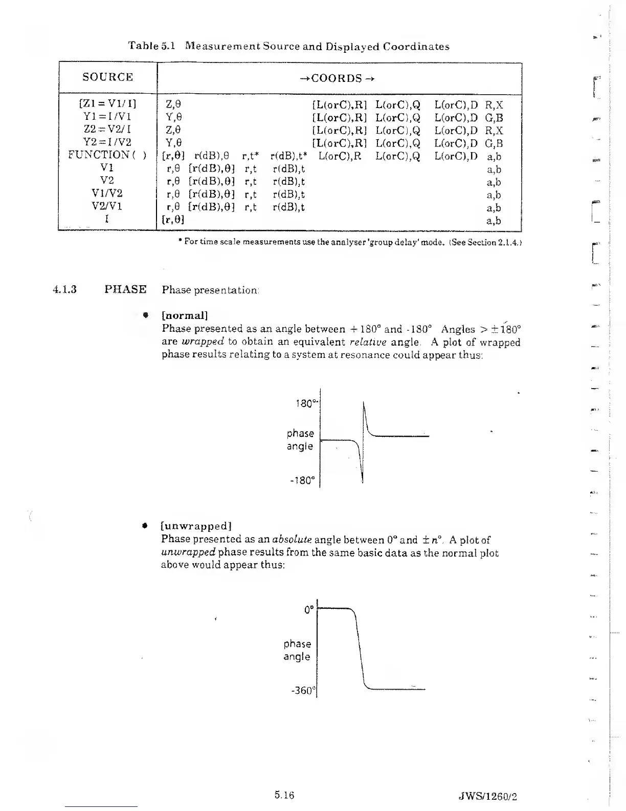
* [normal]
Phase presented
as an angle between
4-
180°
and
-180°
Angles >
±
180°
are wrapped to obtain
an equivalent
relative angle.
A
plot
of wrapped
phase results relating to
a system
at resonance could
appear thus:
180°*
phase
angle
-180°
•
[unwrapped]
Phase
presented as an absolute
angle between
0°
and ± n°. A plot of
unwrapped
phase results from
the
same basic
data as the
normal
plot
above
would appear thus:
5.16
JWS/
1260/2