Redstone™ Optical Spectrum Analyzer Chapter 8: Operation
Page 37 STN053070-D02
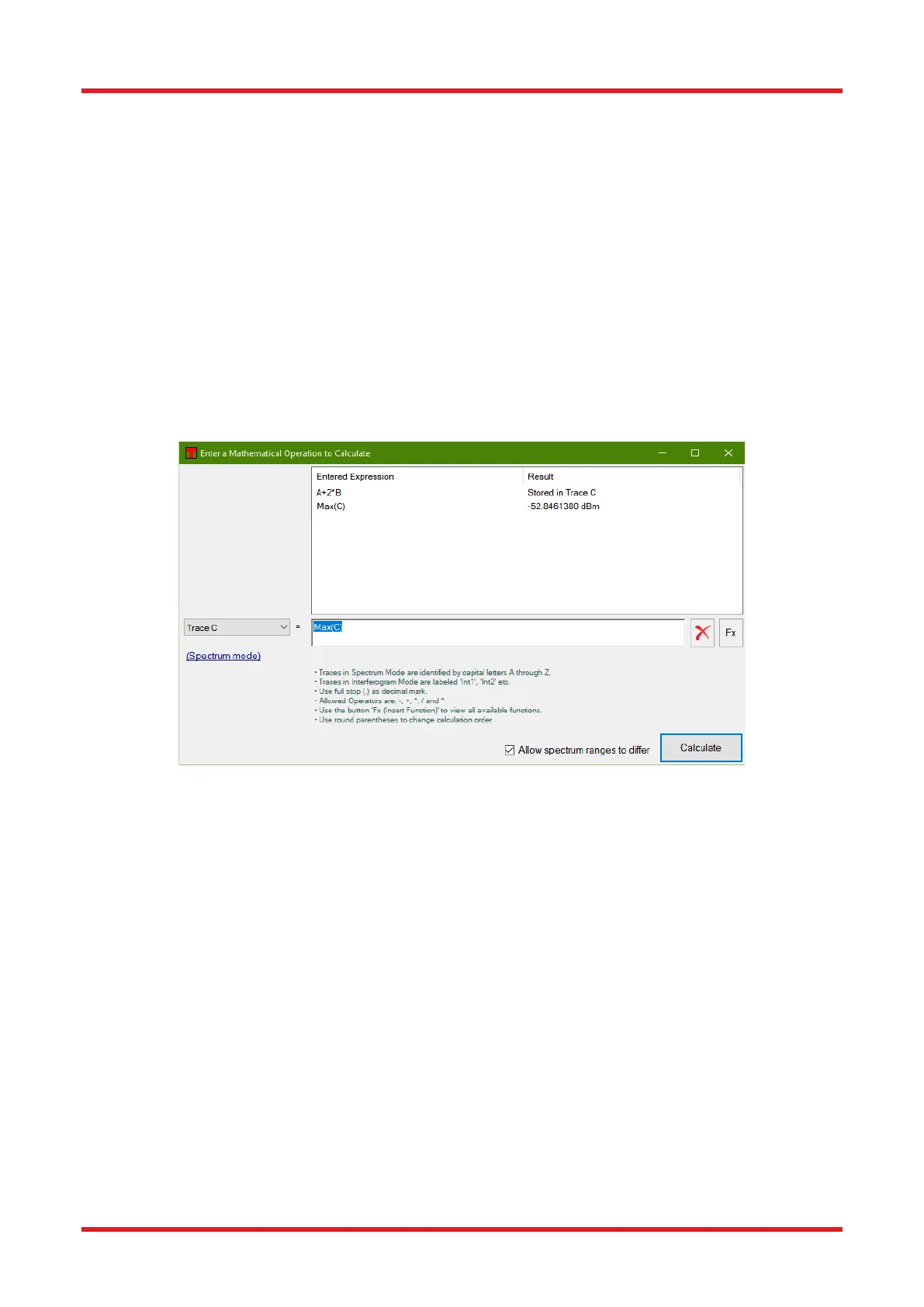
• Spectrum traces are identified by letters A through Z (case insensitive); interferogram traces are
identified by “Int1” through “Int26” (case insensitive). Only the traces which can be seen in the trace
controls bar can be used.
• Use a decimal point (full stop, ‘.’) as decimal mark.
• Allowed operators are: subtraction (‘-’), addition (‘+’), division (‘/’), multiplication (‘*’) and power of (‘^’).
• Operations can be grouped or nested using round parentheses.
The expression can also contain mathematical functions; available functions are listed and inserted by clicking
on the button labelled “Fx.”
The calculation will be performed when the “Calculate” button is clicked or by pressing “Enter” on the keyboard.
If the result of the calculation is a trace, it will be stored in the trace indicated by the drop-down menu in the
dialog box. If the result of the calculation is a scalar, the calculated result will be displayed in the Result section
of the dialog and it will not be saved in a trace.
Figure 36. Mathematical Operations Dialog
Cut: Cuts a trace to a specified region, removing all data outside of that region. A dialog box will open, in which
the exact region and the input/output traces can be specified.
Convolution: Performs a convolution between a trace and one of two kernels: Gaussian and sinc. A dialog box
will open, in which the type and width of kernel and the input/output traces can be specified.
Apodize: Performs an apodization of an interferogram. A dialog box will open, in which the type of apodization
function and the input/output traces can be specified. For more details on apodization, see Sections 4.10 and
16.2. This operation is only available for interferograms.
Invert: Calculates the reciprocal of the Active trace.
Zero Out: Sets all values in a specified region of a trace to zero. A dialog box will open, in which the exact
region and the input/output traces can be specified.
Smooth: Performs a smoothing operation on a trace or a region thereof. A dialog box will open, in which it is
possible to select the smoothing algorithm to use and to set the parameters for the smoothing as well as the
input/output traces.
Curve Fit: Fits a mathematical curve to a trace or a region thereof. A dialog box will open, in which the fit
settings and intput/output traces can be specified. Available math functions are: Gaussian, Lorentzian, and
polynomial, see Section 8.7.7 Functional Traces (Traces Defined by a Function).
 Loading...