Optical Backscatter Reflectometer 4600 55
User Guide
sum of these two spectra is then calculated to generate a polarization-independent
spectrum associated with each fiber segment.
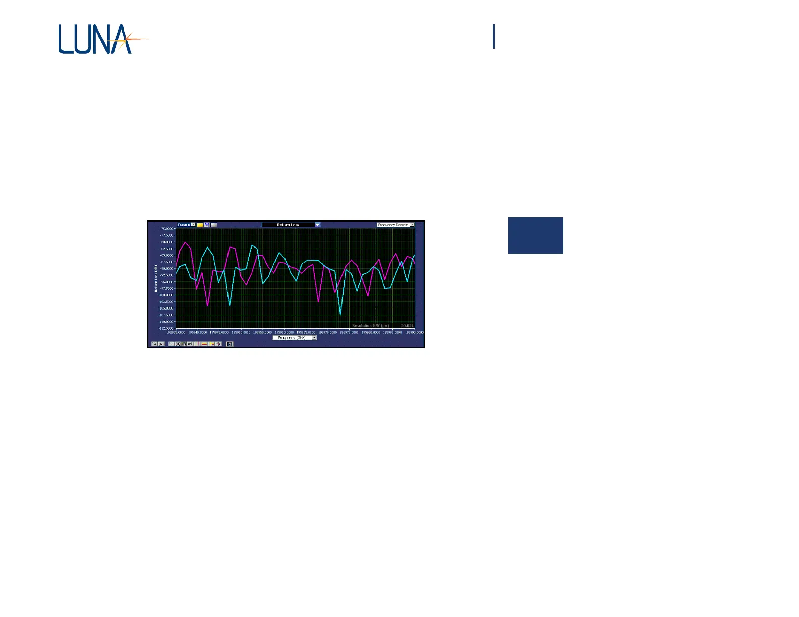
An example of a small spectral shift for the data displayed in Figure 4-9 is shown
in Figure 4-10 below. In this case the lower graph selection options were changed
from Time
Domain
to
Frequency Domain
and from
Spectral
Shift to
Return
Loss,
and the frequency axis scale was reduced to show close-up detail of the spectral
signatures of Traces A (blue) and E (purple). Trace A appears as a similar version
of Trace E, shifted in frequency by +5 GHz, consistent with the spectral shift result
in Figure 4-9.
4
Figure 4-10. Close-up of a part of the spectrum for the yellow cursor in Figure 4-9.
Trace A (blue) and Trace E (purple—the Shift Reference) exhibit similar
features, but Trace A is shifted roughly 5 GHz to the right of Trace E.
Figures 4-11 and 4-12 show temporal shift results for a different section of the FUT
data shown in the upper
window
of Figure 4-9. The
temporal
shift
displayed
in Figure
4-11 agrees well with the
observed
shift in the
temporal
return loss
amplitude
patterns
for Traces A and E shown in Figure 4-12.