Solver NEXT SPM. Instruction Manual
166
2) Pulse shape . The applied force gets its maximum level A1 instantly and then the
force remains constant for the time t. After the time t expires the force returns to the
level А0.
3) Pulse shape . The time interval t is divided by three equal parts (see Fig. 8-3). Initial
level of the applied force is А0. The applied force ramps linearly during the first part
(of duration t/3), to the level А1 and remains constant for the next subinterval t/3.
Finally, during the last subinterval t/3 the force returns to its initial level А0.
4) Pulse shape . The applied force ramps linearly to the level A1 during the time t.
After the time t expires the force returns to the level А0.
5) Pulse shape . The applied force gets the level A1 instantly. Then, during the time t
the force returns linearly to its initial level А0.
6) Pulse shape . The time interval t is divided by two equal parts. The applied force
ramps linearly to level A1 during time t/2 and then remains constant during the second
subinterval t/2. After the time t/2 expires the force returns to the level А0.
7) Pulse shape . The time interval t is divided by two equal parts. The applied force
gets its maximum level A1 instantly and then the force remains constant for the time
t/2. Finally, during the subinterval t/2 the force returns to its initial level А0.
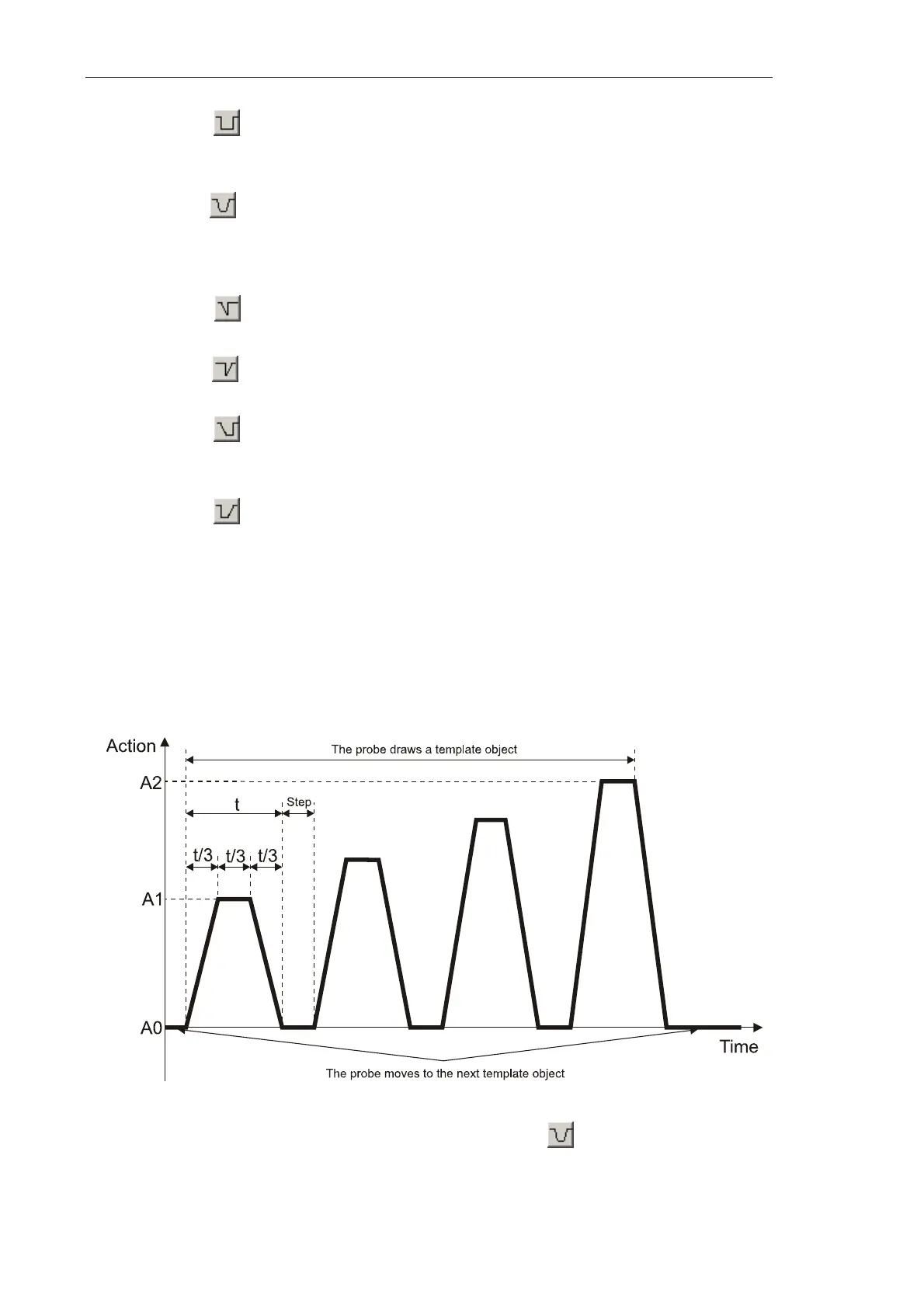
8.1.1.4. Pulse-gradient lithography
Pulse-gradient lithography is a combination of two modifications of lithography, the pulse
and the gradient ones. The Figure below demonstrates a time diagram of the force applied
to the sample in the course of the Pulse-gradient lithography(Fig. 8-5).
Fig. 8-5. Force applied to the sample in the course of the Pulse-gradient lithography.
Example of the pulse shape is shown