NT-MDT Solver Next - Approaching the Sample to the Probe; Adjusting Working Level of the Feedback Gain; Adjusting Scanning Parameters; Scanning

Solver NEXT SPM. Instruction Manual
72
7.1.2.2. Procedural Sequence
Procedures of the Lateral Force Mode are based on those of the Constant Force Mode that
is described in detail in sect. 7.1.1 “Constant Force Mode” on p. 55.
Main procedures involved in the Lateral Force Mode
1. Adjusting the Controller Configuration (see i. 7.1.1.1 on p. 56).
2. Adjusting Initial Level of the DFL Signal (see i. 7.1.1.1 on p. 56).
3. Approaching the Sample to the Probe (see i. 7.1.1.2 on p. 56).
4. Adjusting Working Level of the Feedback Gain (see i. 7.1.1.3 on p. 58).
5. Adjusting Scanning Parameters (see i. 7.1.1.4 on p. 60).
6. Scanning (see i. 7.1.1.5 on p. 62).
7. Saving Measurement Data (see i 7.1.1.6 on p. 66).
8. Completing Measurements (see i 7.1.1.7 on p. 70).
7.1.2.3. Scanning
The basic difference of operation in this mode from that of the Constant Force Mode is in
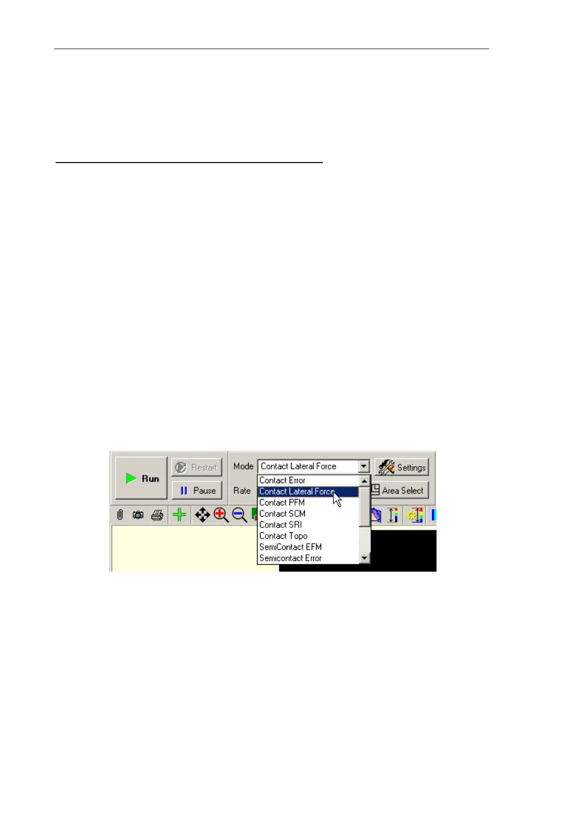
the step of item. 7.1.1.5 “Scanning” on p. 62 (see sect. “Selecting AFM mode” on p. 62)
where the Contact Lateral Force option in the Mode list should be selected instead of
Contact Topo (see Fig. 7-27). This selection provides proper automatic electronic
arrangement required by the mode.
Fig. 7-27. Selecting the Lateral Force Microscopy
To start scanning, click the Run button in the Control panel of the Scanning window.
This launches line-by-line scanning of the sample surface and the 2D Viewer of the scan
data will display three 2D data views. The first view shows the surface landscape (Height
signal) while the other two display distributions of the lateral force (LF signal)
(see Fig. 7-28) detected in forward and backward sweeps of the scan lines.