Chapter 7. Performing Measurements
157
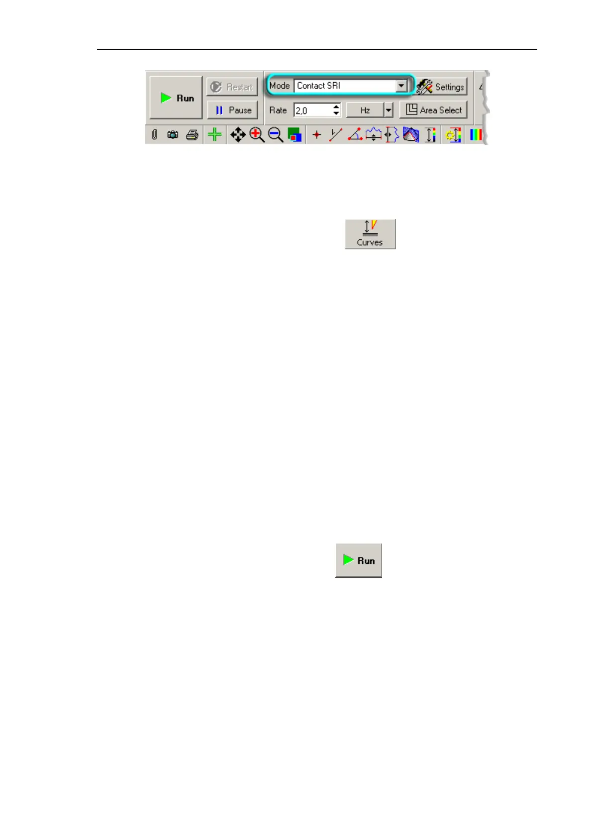
Fig. 7-146
The instrument will be automatically reconfigured for the selected measurement mode.
3. Open the spectroscopy window by clicking the button.
4. In the
Spectroscopy Mode drop-down list, select I(V) AFM. This will result in:
● selecting the IProbe signal as a recorded signal in the Measurements panel;
● selecting the BV Value signal as the argument of the measured relation in the
Argument panel.
Redefine the set of measured signals, if necessary.
5. In the fields From and To, define the variation range of the argument of the measured
relation.
NOTE. If the
Rel
option is selected in the drop-down list of the
Argument
panel, the
origin of coordinates will taken at the
BV
level defined in the Main Parameters panel.
Otherwise, if the
Absolute
option is selected,
BV
= 0 is assumed for the coordinate
origin.
6. Define the desired limits for a signal if necessary.
7. In the Speed group, adjust speeds of taking 1D relations at forward (Forw parameter)
and backward (Back parameter) scanning.
8. Select the mode of defining the spectroscopy points (by points, by a line, or by a grid)
and define the points.
9. Launch measurements by clicking the button .
When the measurements complete, the Viewing Area displays a plot for the last
measurement point. A typical plot of the
I(V) relation is shown in Fig. 7-147.