Statistics 12–7
82D315~1.DOC TI-83 international English Bob Fedorisko Revised: 10/26/05 1:36 PM Printed: 10/27/05 2:53
PM Page 7 of 38
The residual pattern indicates a curvature associated with this data set for which the
linear model did not account. The residual plot emphasizes a downward curvature, so
a model that curves down with the data would be more accurate. Perhaps a function
such as square root would fit. Try a power regression to fit a function of the form y =
a ä x
b
.
22. Press o to display the Y= editor.
Press ‘ to clear the linear regression
equation from
Y1. Press } Í to turn on
plot 1. Press ~ Í to turn off plot 2.
23. Press q 9 to select 9:ZoomStat from the
ZOOM menu. The window variables are
adjusted automatically, and the original
scatter plot of time-versus-length data (plot
1) is displayed.
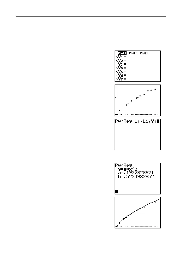
24. Press … ~ ƒ [A] to select
A:PwrReg from the STAT CALC menu.
PwrReg is pasted to the home screen.
Press y [L1] ¢ y [L2] ¢. Press
~
1 to display the VARS Y.VARS
FUNCTION
secondary menu, and then press
1 to select 1:Y1. L1, L2, and Y1 are pasted to
the home screen as arguments to
PwrReg.
25. Press Í to calculate the power
regression. Values for
a and b are displayed
on the home screen. The power regression
equation is stored in
Y1. Residuals are
calculated and stored automatically in the
list name
RESID.
26. Press s. The regression line and the
scatter plot are displayed.

 Loading...