Chapter 7. Performing Measurements
155
samples this assumption is fairly realistic. Therefore, the Δ Height range corresponding to
the variation of the Mag signal from its initial level (equal to Set Point) to zero will be
equal to the cantilever oscillations amplitude.
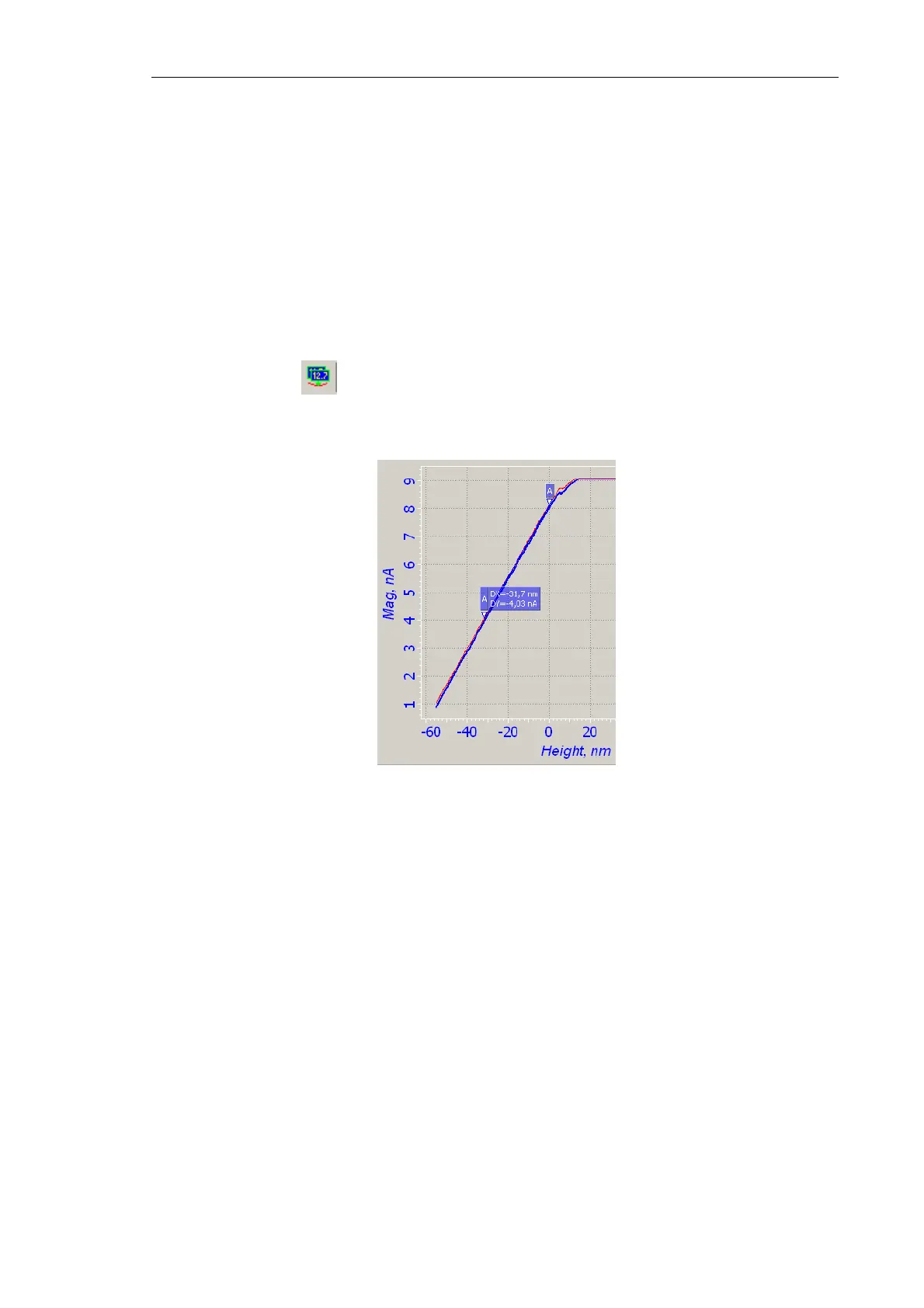
As seen from the spectroscopy data, the sloped part of the curve has a region with linear
variation of Mag against Height:
Δ
Height = K ×
Δ
Mag, (2)
where K – is proportionality constant.
To calculate the calibration coefficient measure the values of Δ Mag and Δ Height. To this
purpose, press the button (Pair Markers) in the 1D Data Viewer and place the two
markers on the inclined portion of the curve (Fig. 7-144). The values of DX and DY
measured using the markers are Δ Height and Δ Mag, respectively.
Fig. 7-144
Thus, following equation (2) the proportionality constant connecting the cantilever
oscillations amplitude with the value of the
Mag signal is given by:
K =
Δ
Height /
Δ
Mag = DX / DY= 31.7 / 4 = 7.93 [nm/nA]. (3)
The actual amplitude of the cantilever oscillations can be calculated from the following
equation:
Amplitude = K×Mag. (4)
In the example, when performing a scan with the parameter Set Point = 8 nA, the
amplitude of oscillations is 64 nm.