Appendix B: Technical Reference 938
Contour Levels and Implicit Plot Algorithm
Contours are calculated and plotted by the following method. An implicit plot is the same
as a contour, except that an implicit plot is for the z=0 contour only.
Algorithm
Based on your x and y Window variables, the distance between xmin and xmax and
between ymin and ymax is divided into a number of grid lines specified by xgrid and
ygrid. These grid lines intersect to form a series of rectangles.
The
E value is treated as the value of the equation at the center of the rectangle.
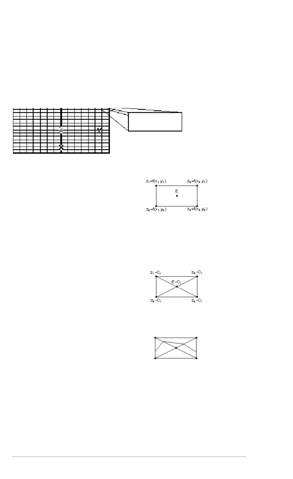
For each specified contour value (Ci)
Each rectangle in the grid is treated similarly.
Runge-Kutta Method
For Runge-Kutta integrations of ordinary differential equations, the TI-89 Titanium /
Voyage™ 200 uses the Bogacki-Shampine 3(2) formula as found in the journal Applied
Math Letters, 2 (1989), pp. 1–9.
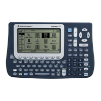
For each rectangle, the equation is evaluated at
each of the four corners (also called vertices or
grid points) and an average value (E) is
calculated:
E =
• At each of the five points shown to the right,
the difference between the point’s z value
and the contour value is calculated.
• A sign change between any two adjacent points implies that a contour crosses the line that
joins those two points. Linear interpolation is used to approximate where the zero crosses
the line.
• Within the rectangle, any zero crossings
are connected with straight lines.
• This process is repeated for each contour
value.
z1 z2 z3 z4+++
4
-----------------------------------------
 Loading...