238 WM-OM-E Rev I
the dBm scale, with 0 dBm corresponding to (V
ref
2
/Hz).
Sampling Frequency The time-domain records are acquired at sampling frequencies dependent
on the selected time base. Before the FFT computation, the time-domain record may be decimated.
If the selected maximum number of points is lower than the source number of points, the effective
sampling frequency is reduced. The effective sampling frequency equals twice the Nyquist
frequency.
Scallop Loss This is loss associated with the picket fence effect.
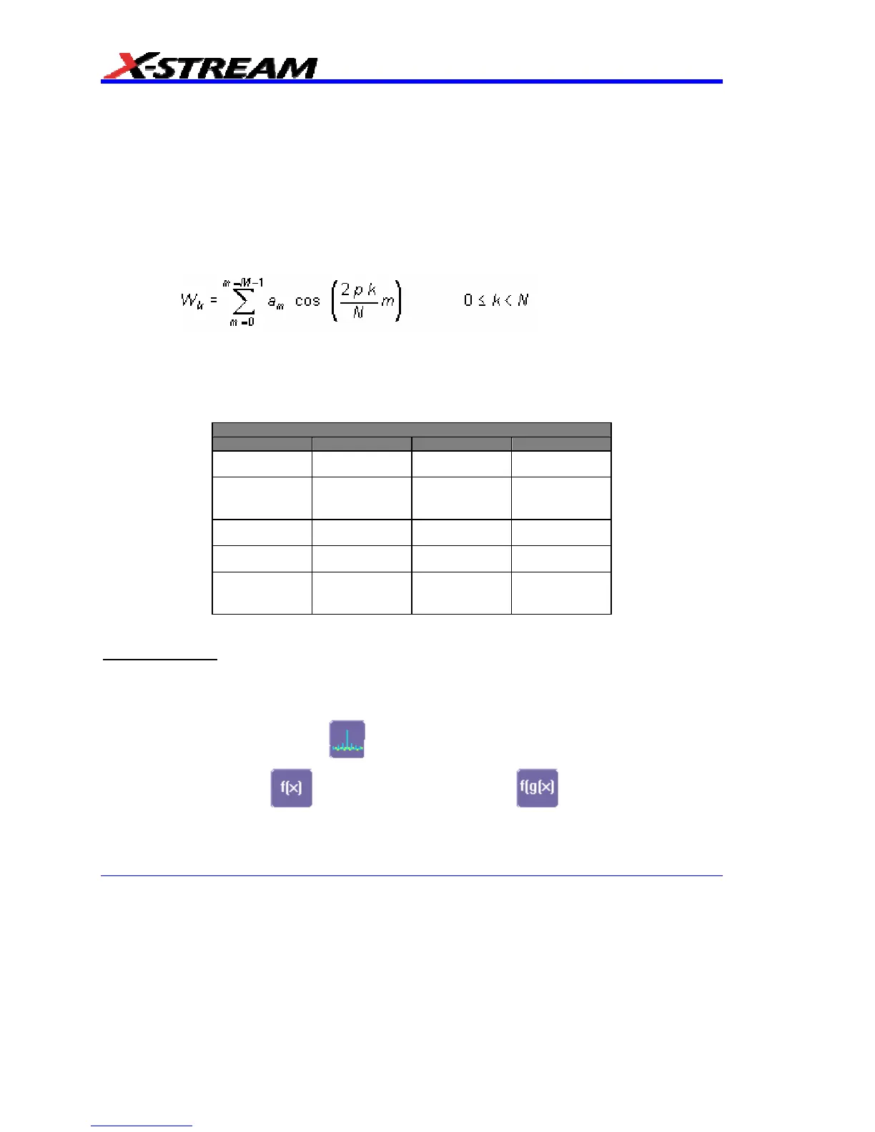
Window Functions All available window functions belong to the sum of cosines family with one to
three non-zero cosine terms:
where: M = 3 is the maximum number of terms, a
m
are the coefficients of the terms, N is the number
of points of the decimated source waveform, and k is the time index.
The table of Coefficients of Window Functions lists the coefficients a
m
. The window functions seen
in the time domain are symmetric around the point k = N/2.
Coefficients of Window Functions
Window Type a
0
a
1
a
2
Rectangular
1.0 0.0 0.0
Hanning (Von
Hann)
0.5 -0.5 0.0
Hamming
0.54 -0.46 0.0
Flattop
0.281 -0.521 0.198
Blackman-Har
ris
0.423 -0.497 0.079
FFT Setup
To Set Up an FFT
1. In the menu bar touch Math, then Math Setup... in the drop-down menu.
2. Touch a Math function trace button: F1 through Fx The number of math traces available
depends on the software options loaded on your scope. See Specifications.; a pop-up
menu appears. Select FFT
from the menu.
3. Touch the Single
or Dual (function of a function) button if the FFT is to be
of the result of another math operation.
4. Touch inside the Source1 field and select a channel, memory, or math trace on which to
perform the FFT.