Data Processing Algorithms
276 0112-0109 H
Each well-specific spatial uniformity correction factor is calculated by
dividing the mean fluorescence counts of all wells by the fluorescence
counts of each well (taken at Sample 1.) The table above also presents
the correction factor for wells A1–A9.
All samples taken from a particular well are multiplied by their well-
specific correction factor. For example, all samples from A1 are
multiplied by 1.12, A2 by 1.05, etc.
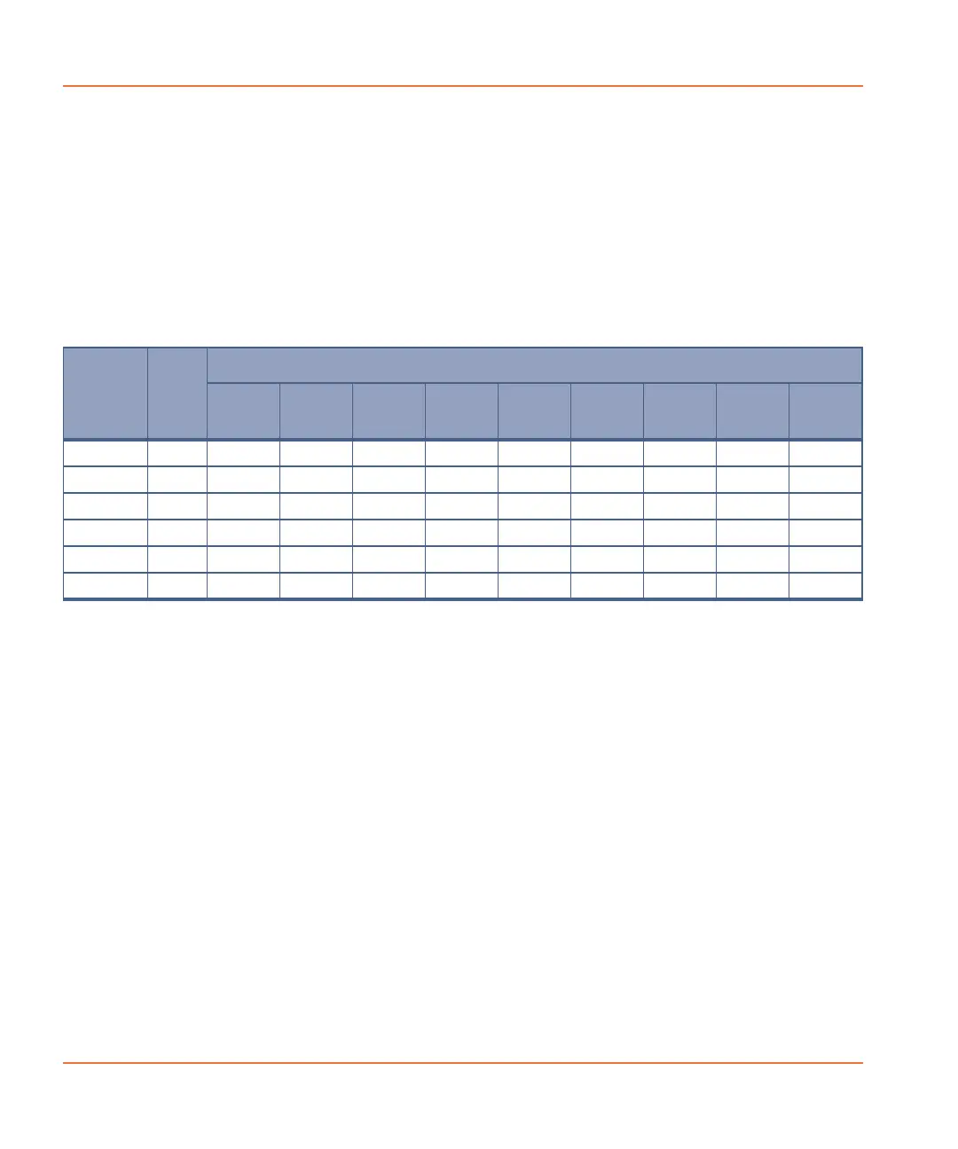
The results of applying the spatial uniformity correction factor are
presented in the table below. Note the decreased variability range of
wells A1–A9 in Sample 1 (8900–8976) as compared to the same data
prior to applying the correction algorithm (8000–10000).
If the spatial uniformity correction factor is applied to plates with empty
wells, non dye-loaded cells, or a panel of cells containing different dyes
and/or dye concentrations, the well-specific fluorescence counts will be
skewed by the correction factor. However, the EC
50
of the agonists
tested will not be affected.
Negative Control Correction
The negative control correction algorithm corrects for changes in
fluorescence that occur in all wells over the course of the experiment.
Causes for these changes in fluctuations in fluorescence include dye
leakage from cells, fluid addition artifacts, changes in illumination
power, dye photo-bleaching, and temperature drifts.
Sample Time
Well
A1
– Ctr
A2
– Ctrl
A3
– Ctrl
A4
Exp
A5
Exp
A6
Exp
A7
+ Ctrl
A8
+ Ctrl
A9
+ Ctrl
1 0 8960 8925 8930 8938 8924 8976 8900 8930 8961
2 5 9194 9030 8836 9047 8730 9180 8455 9118 9270
3 10 9408 8925 8648 9265 8730 9282 8633 9118 9682
4 20 9632 8820 8648 49050 48500 42840 50730 48880 55620
5 25 9632 9240 8648 40330 40740 35700 47170 47000 51500
6 30 9856 8925 8930 32700 33950 29580 44500 47940 51500
 Loading...