TI-83, TI-83 Plus, TI-84 Plus Guide
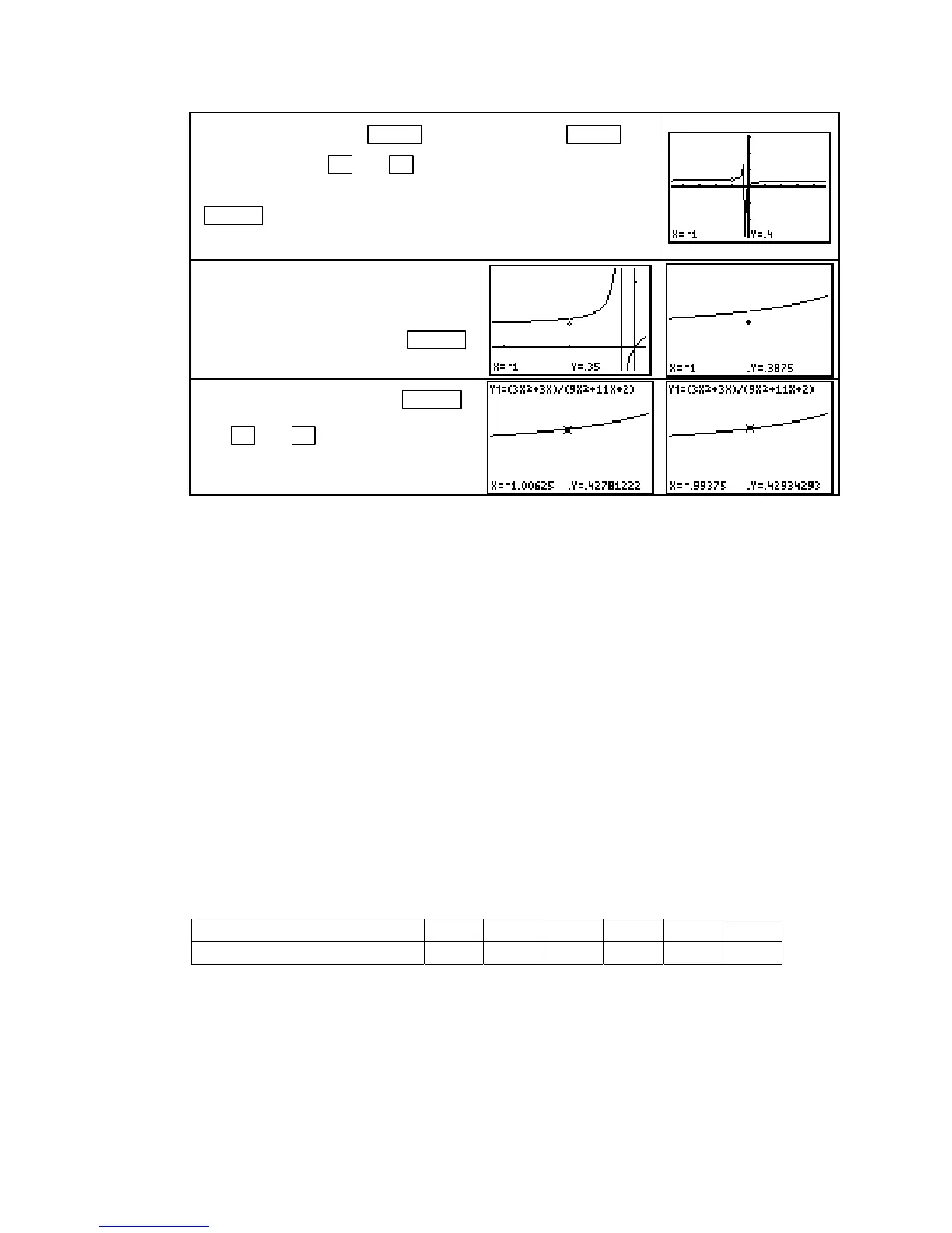
Draw a graph of h with
ZOOM 4 [ZDecimal]. Press ZOOM 2
[Zoom In]
and use ◄ and ▲ to move the blinking cursor
until you are near the point on the graph where x =
−
1. Press
ENTER . If you look closely, you can see the hole in the graph
at x =
−
1. (Note that we are not tracing the graph of h.)
If the view is not magnified enough to
see what is happening around x =
−
1,
have the cursor near the point on the
curve where x =
−
1 and press ENTER
to zoom in again.
To estimate
lim
x→
−
1
h(x), press TRACE ,
use
► and ◄ to trace the graph
close to, and on either side of x =
−
1,
and observe the sequence of y-values.
Observing the sequence of y-values is the same procedure as numerically estimating the limit at
a point. Therefore, it is not the value at x =
−
1 that is important; the limit is what the output
values displayed on the screen approach as x approaches
−
1. It appears that
lim
x→
−
1
−
h(x) ≈ 0.43
and
lim
x→
−
1
+
h(x) ≈ 0.43. Therefore, we conclude that
lim
x→
−
1
h(x) ≈ 0.43.
1.5 Polynomial Functions and Models
You will in this section learn how to fit functions that have the familiar shape of a parabola or
a cubic to data. Using your calculator to find these equations involves the same procedure as
when using it to fit linear, exponential, log, or logistic functions.
FINDING SECOND DIFFERENCES When the input values are evenly spaced, you can
use program
DIFF to quickly compute second differences in the output values. If the data are
perfectly quadratic (that is, every data point falls on a quadratic function), the second differ-
ences in the output values are constant. When the second differences are close to constant, a
quadratic function may be appropriate for the data.
We illustrate these ideas with the roofing jobs data given in Table 1.26 of Section 1.5 in
Calculus Concepts. We align the input data so that 1 = January, 2 = February, etc. Clear any
old data and enter these data in lists
L1 and L2:
Month of the year 1 2 3 4 5 6
Number of roofing jobs 90 91 101 120 148 185
The input values are evenly spaced, so we can see what information is given by viewing the
second differences.
Copyright © Houghton Mifflin Company. All rights reserved.
39

 Loading...


