TI-83, TI-83 Plus, TI-84 Plus Guide
Chapter 10 Analyzing Multivariable Change:
Optimization
10.2 Multivariable Optimization
As you might expect, multivariable optimization techniques that you use with your calculator
are very similar to those that were discussed in Chapter 4. The basic difference is that the
algebra required to get the expression that comes from solving a system of equations with
several unknowns reduced to one equation in one unknown is sometimes difficult. However,
once your equation is of that form, all the optimization procedures are basically the same as
those that were discussed previously.
10.2.1 FINDING CRITICAL POINTS USING ALGEBRA AND THE SOLVER Critical
points for a multivariable function are points at which maxima, minima, or saddle points
occur. We begin the process of finding critical points of a smooth, continuous multivariable
function by using derivative formulas to find the partial derivative with respect to each input
variable and setting these partial derivatives each equal to 0. We next use algebraic methods
to obtain one equation in one unknown input. Then, you can use your calculator’s solver to
obtain the solution to that equation. This method of solution works for all types of equations.
We illustrate these ideas with the postal rate function given at the beginning of Section 10.2:
The volume of a rectangular package that contains the maximum amount of printed
material and is sent at the bound printed matter postal rate is given by
V(h, w) = 108hw – 2h
2
w – 2hw
2
cubic inches
where h inches is the height and w inches is the width of the package.
Find the two partial derivatives and set each of them equal to 0 to obtain these equations:
V
h
: 108w – 4hw – 2w
2
= 0 [1]
V
w
: 108h – 2h
2
– 4hw = 0 [2]
WARNING: Everything that you do with your calculator depends on the partial derivative
formulas that you find using derivative rules.
Next, solve one of the equations for one of the variables, say equation 2 for w, to obtain
w =
108 2
4
2
hh
h
−
Remember that to solve for a quantity means that it must be by itself on one side of the equa-
tion without the other side of the equation containing that letter. Now, let your calculator
work.
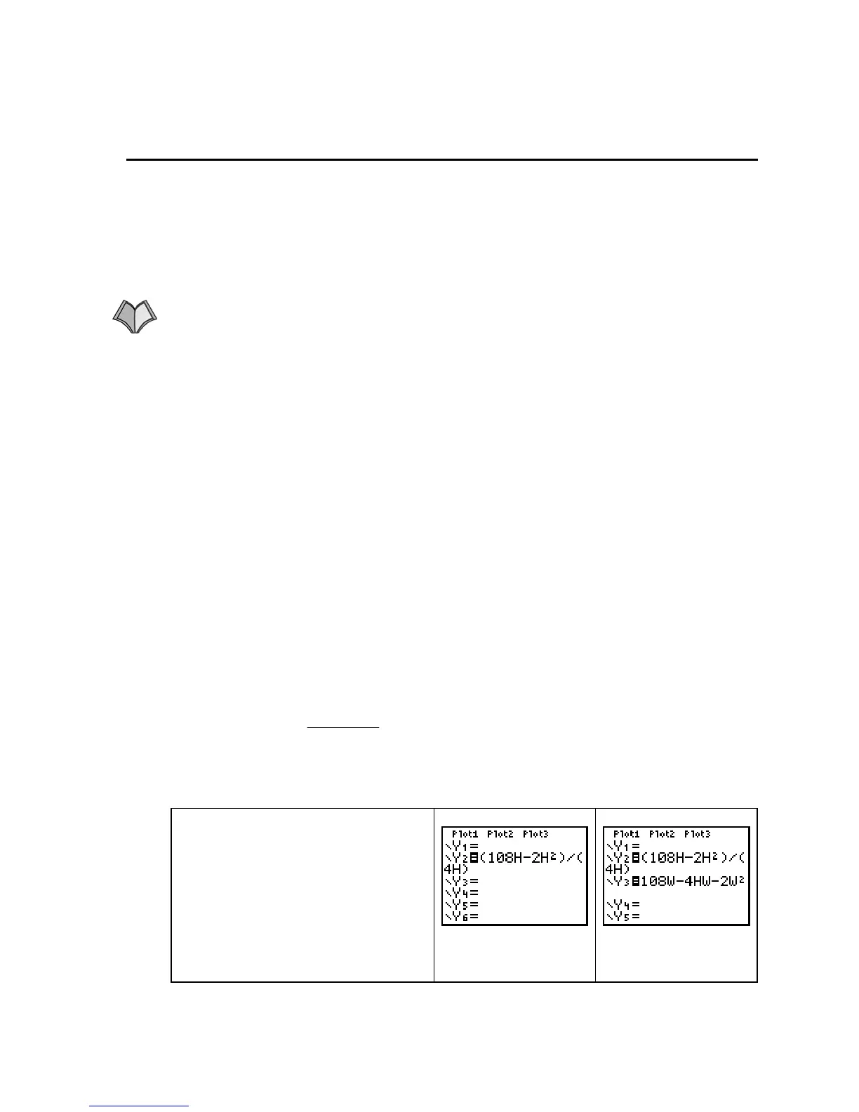
Clear the Y= list. Enter the expression
for w in
Y2. Be certain that you en-
close numerators and denominators of
fractions in parentheses. (We later
enter the function V in
Y1.)
Type the left-hand side of the other
equation (here, equation 1) in
Y3. (The
expression you type in
Y3 must be
equal to zero.)
This step tells the
calculator that w = Y2.
Equations 1 and 2 are
now in the calculator.
Copyright © Houghton Mifflin Company. All rights reserved.
105

 Loading...


