TI-83, TI-83 Plus, TI-84 Plus Guide
The slope
dy/dx = 2.0666667 appears at the bottom of the screen.
Return to the home screen and press X,T,θ,n . The calculator’s
X memory location has been updated to 3. Now type the
numerical derivative instruction (evaluated at 3) as shown to the
right. This is the
dy/dx value you saw on the graphics screen.
You can use the ideas presented above to check your algebraic formula for the derivative. We
next investigate this procedure.
NUMERICALLY CHECKING SLOPE FORMULAS It is always a good idea to check
your answer. Although your calculator cannot give you an algebraic formula for the derivative
function, you can use numerical techniques to check your algebraic derivative formula. The
basic idea of the checking process is that if you evaluate your derivative and the calculator’s
numerical derivative at several randomly chosen values of the input variable and the outputs
are basically the same values, your derivative is
probably correct.
These same procedures are applicable when you check your results (in the next several
sections) after applying the Sum Rule, the Chain Rule, or the Product Rule. We use the fun-
ction in part
c of Example 2 in Section 3.3 of Calculus Concepts to illustrate.
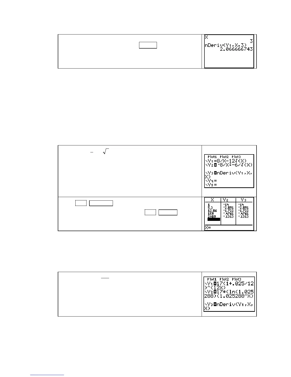
Enter m(r) =
8
12
r
r− in Y1 (using X as the input variable).
Compute m′(r) using pencil and paper and the derivative rules.
Enter this function in
Y2. (What you enter in Y2 may or may
not be the same as what appears to the right.)
Enter the calculator’s numerical derivative of
Y1 (evaluated at a
general input
X) in Y3. Because you are interested in seeing
if the outputs of
Y2 and Y3 are the same, turn off Y1.
Press 2ND WINDOW (TBLSET) and choose ASK in the
Indpnt: location. Access the table with 2ND GRAPH (TABLE)
and delete or type over any previous entries in the X column.
Enter at least three different values for
X.
The table gives strong evidence that that Y2 and Y3 are the same function.
GRAPHICALLY CHECKING SLOPE FORMULAS When it is used correctly, a graphi-
cal check of your algebraic formula works well because you can look at many more inputs
when drawing a graph than when viewing specific inputs in a table. We illustrate this use with
the function in part d of Example 2 in Section 3.3 of Calculus Concepts.
Enter j(y) =
()
12
0.025
12
17 1
y
+ in Y1, using X as the input variable.
Next, using pencil and paper and the derivative rules, compute
j
′
(y). Enter this function in Y2.
Enter the calculator’s numerical derivative of
Y1 (evaluated at a
general input
X) in Y3. Before proceeding, turn off the graphs
of
Y1 and Y3.
To graphically check your derivative formula answer, you now need to find a good graph of
Y2. Because this function is not in a context with a given input interval, the time it takes to
find a graph is shortened if you know the approximate shape of the graph. Note that the graph
of the function in
Y2 is an increasing exponential curve.
Copyright © Houghton Mifflin Company. All rights reserved.
57

 Loading...


