TI-83, TI-83 Plus, TI-84 Plus Guide
CONSUMER ECONOMICS We illustrate how to find the consumers’ surplus and other
economic quantities when the demand function intersects the input axis as given in Example 1
of Section 6.3 of Calculus Concepts:
Suppose the demand for a certain model of minivan in the United States can be
described as D(p) = 14.12(0.933
p
) – 0.25 million minivans when the market price
is p thousand dollars per minivan.
We first draw a graph of the demand function. This is not asked for, but it will really help
your understanding of the problem. Read the problem to see if there are any clues as to how to
set the horizontal view for the graph. The price cannot be negative, so p
≥ 0. There is no price
given in the remainder of the problem, so just guess a value with which to begin.
Enter D in Y1, using X as the input variable. Press WINDOW ,
set
Xmin = 0 and we choose Xmax = 20 (remember that the price
is in thousands of dollars). Use
ZOOM ▲ [ZoomFit] to draw
a graph. Reset
Ymin = 0 and press GRAPH .
Even though D is an exponential function, a constant has been
subtracted from the exponential portion. So, D may cross the
input axis. Notice that if it does, the x-intercept will be greater
than 20. You could try different values for
Xmax, but we choose
to use the
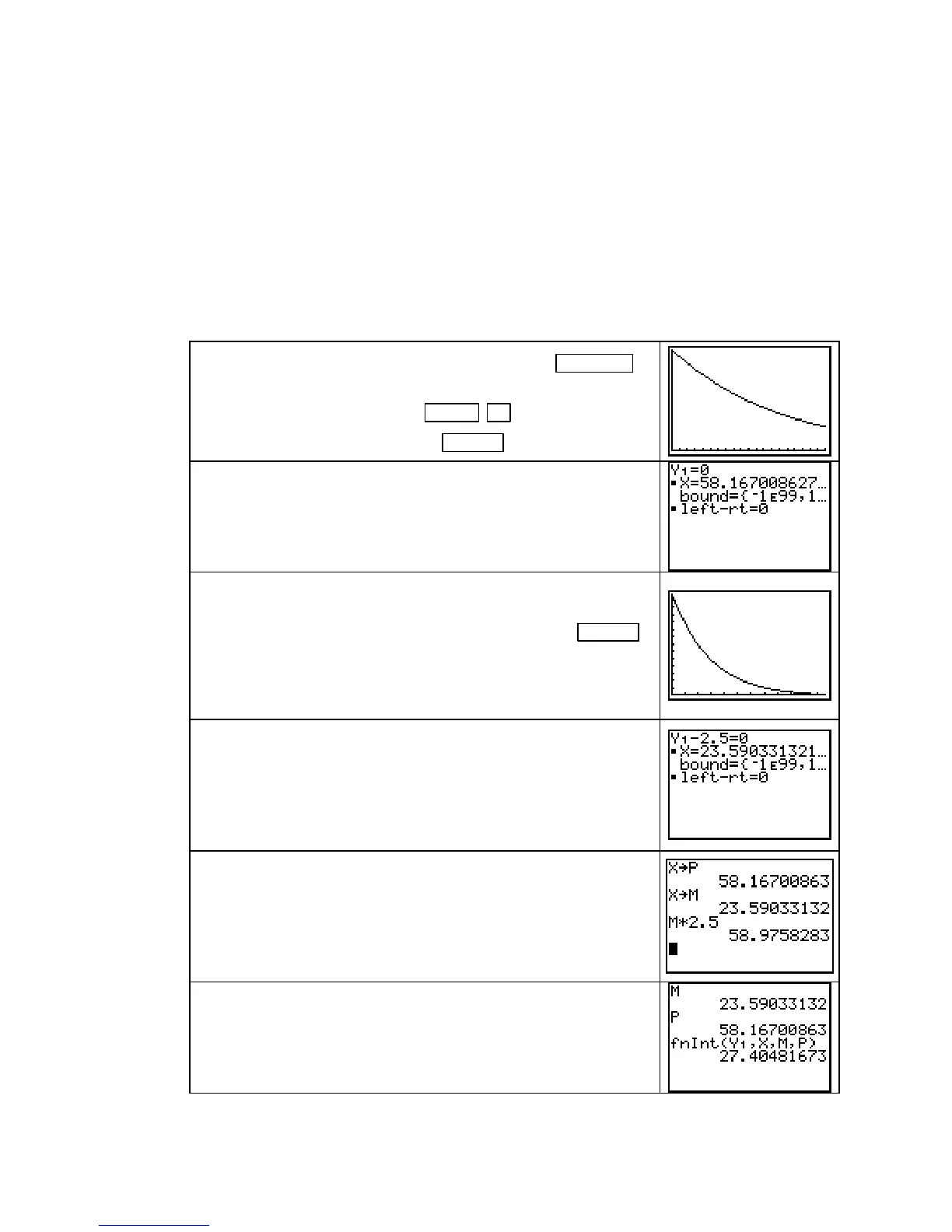
SOLVER to see if there is a value such that Y1 = 0.
Customers will not purchase this model minivan if the price per
minivan is more than about $58.2 thousand. Store this value in P
for later use and set
Xmax = P. Redraw the graph with GRAPH .
(Be sure to label the axes with variables and units of measure
when you copy this graph to your paper.)
Note that the answer to Example 1, part c, is p ≈ $58.2 thousand.
Part a of Example 1 asks at what price consumers will purchase
2.5 million minivans. Look at the labels on your graph and note
that 2.5 is a value of D, not
p. You therefore need to find the
price (an input). Return to the solver and edit the equation so to
solve
Y1 − 2.5 = 0. You can trace the graph for a guess, but
there is only one answer, so any reasonable guess will suffice.
Part b asks for the consumers’ expenditure when purchasing 2.5
million minivans. First, store this market price in M for future
use. (Also label this value M on your hand-drawn graph.) The
consumers’ expenditure is price * quantity = area of the rectan-
gle with height = 2.5 million minivans and width
≈ $23.59
thousand per minivan. The area is about $59 billion.
The consumer’s surplus in part d of Example 1 is the area under
the demand curve to the right of M (M
≈ 23.5903) and to the left
of P (P
≈ 58.1670). The surplus is about $27.4 billion.
Copyright © Houghton Mifflin Company. All rights reserved.
85

 Loading...


