TI-83, TI-83 Plus, TI-84 Plus Guide
Chapter 8 Dynamics of Change: Differential
Equations and Proportionality
8.3 Numerically Estimating by Using Differential
Equations: Euler’s Method
Many of the differential equations we encounter have solutions that can be found by determin-
ing an antiderivative of a given rate-of-change function. Thus, many of the techniques that we
learned using the calculator’s numerical integration function apply to this chapter. (See
Chapter 5 of this Guide.)
8.3.1 EULER’S METHOD FOR A DIFFERENTIAL EQUATION WITH ONE INPUT
VARIABLE You may encounter a differential equation that cannot be solved by standard
methods and you may need to draw an accumulation graph for a differential equation without
first finding an antiderivative. In either of these cases, numerically estimating a solution using
Euler’s method is helpful. This method relies on the use of the derivative of a function to
approximate the change in that function. Recall from Section 4.1 of Calculus Concepts that
the approximate change in a function f at a point is the rate of change of f at that point times a
small change in x. That is,
f(x + h) – f(x) ≈ f
′
(x)
.
h where h represents the small change in x
Now, if we let b = x + h and x = a, the above expression becomes
f(b) – f(a) ≈ f
′
(a)
.
(b – a) or f(b) ≈ f(a) + (b – a)
.
f
′
(a)
The starting values for the coordinates of the point (a, b) will be given to you and are often
called the initial condition. The next step is to repeatedly apply the formula given above to
use the slope of the tangent line at x = a to approximate the change in the function between the
inputs a and b. When h, the distance between a and b, is fairly small, Euler’s method will
often give close numerical estimates of points on the solution to the differential equation
containing f
′
(x).
WARNING: Be wary of the fact that there is some error involved in each step of the Euler
approximation process that is compounded when each result is used to obtain the next result.
We illustrate Euler’s method for a differential equation containing one input variable with
the differential equation in Example 1 of Section 8.3. This equation gives the rate of change of
the total sales of a computer product t years after the product was introduced:
dS
dt t
=
+
6544
12
.
.ln( )
billion dollars per year
Because Euler’s method involves a repetitive process, a program that performs the calculations
used to find the approximate change in the function can save you time and eliminate
computational errors and some error in rounding. The download is available at:
http://college.hmco.com/mathematics/latorre/calculus_concepts/3e/students/programs.html
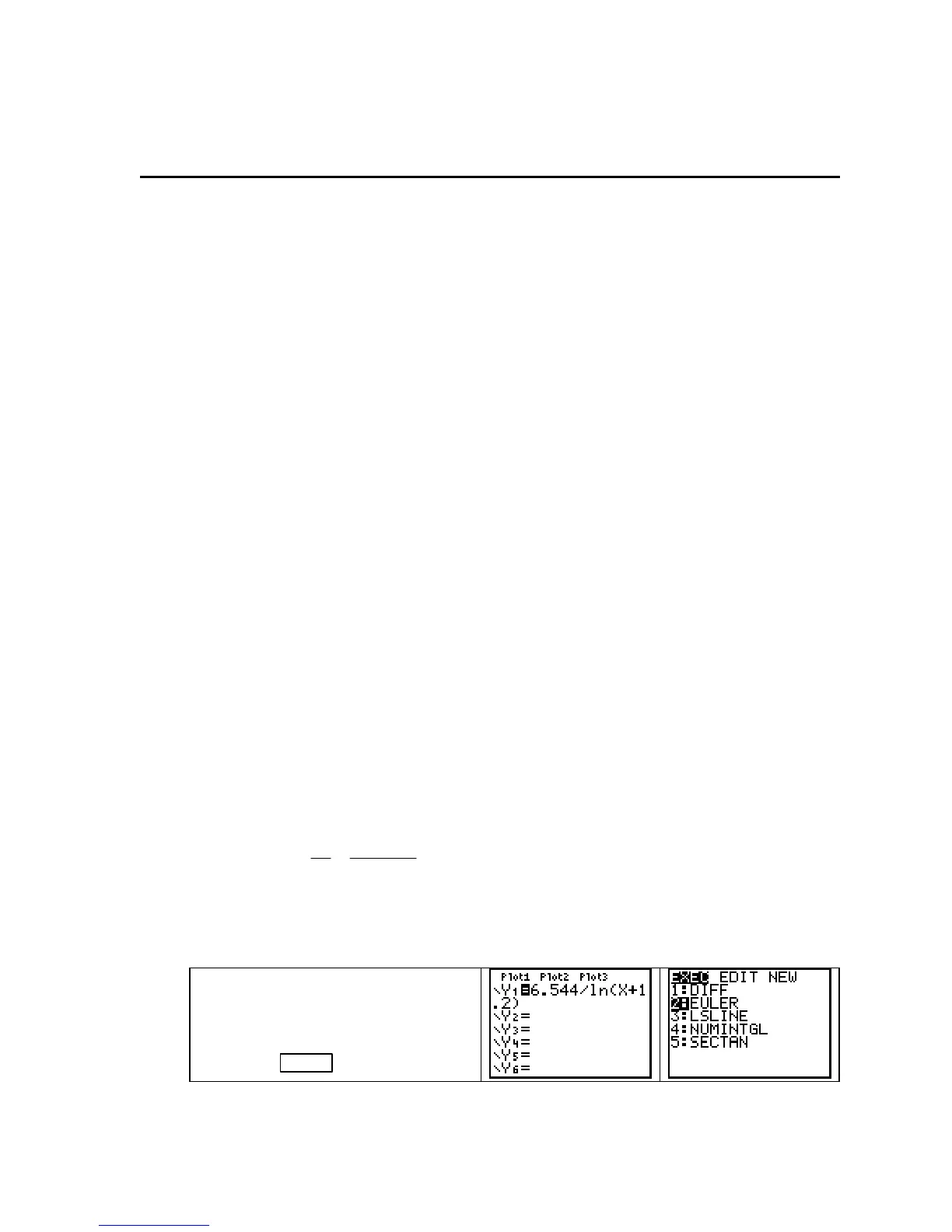
Before using this program, you must
have the differential equation in the
Y1 location of the Y= list with X as
the input variable. Access program
Euler with
PRGM .
Note that your program list may not be the same as the one shown above.
Copyright © Houghton Mifflin Company. All rights reserved.
93

 Loading...


