Chapter 1
Run program
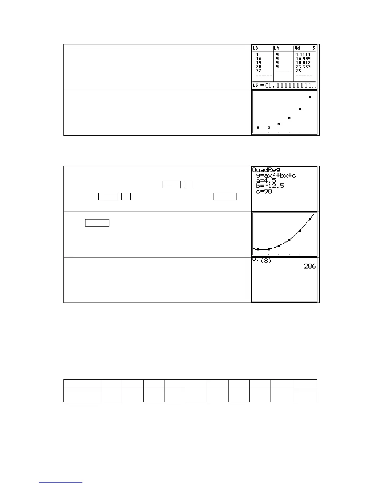
DIFF and observe the first differences in list L3,
the second differences in
L4, and the percentage differences in
list
L5.
The second differences are close to constant, so a quadratic
function may give a good fit for these data.
Construct a scatter plot of the data. (Don’t forget to clear the
Y= list of previously-used equations and to turn on Plot 1.)
The shape of the data confirms the numerical investigation
result that a quadratic function is appropriate.
FINDING A QUADRATIC FUNCTION TO MODEL DATA Use your TI-83 to find a
quadratic function of the form y = ax
2
+ bx + c to model the roofing jobs data.
Find the quadratic function and paste the equation into the Y1
location of the
Y= list by pressing STAT ► [CALC] 5
[QuadReg]
VARS ► [Y−VARS] 1 [Function] 1 [Y1] ENTER .
Press GRAPH to overdraw the graph of the function on the
scatter plot. This function gives a very good fit to the data.
How many jobs do we predict the company will have in August?
Because August corresponds to x = 8, evaluate
Y1 at x = 8. We
predict that there will be 1559 jobs in August.
FINDING A CUBIC FUNCTION TO MODEL DATA Whenever a scatter plot of data
shows a single change in concavity, we are limited to fitting either a cubic or logistic function.
If one or two limiting values are apparent, use the logistic equation. Otherwise, a cubic func-
tion should be considered. When appropriate, use your calculator to obtain the cubic function
of the form y = ax
3
+ bx
2
+ cx + d that best fits a set of data.
We illustrate finding a cubic function with the data in Table 1.30 in Example 3 of Section
1.5 in Calculus Concepts. The data give the average price in dollars per 1000 cubic feet of
natural gas for residential use in the U.S. for selected years between 1980 and 2005.
Year 1980 1982 1985 1990 1995 1998 2000 2003 2004 2005
Price
(dollars)
3.68 5.17 6.12 5.80 6.06 6.82 7.76 9.52 10.74 13.84
Copyright © Houghton Mifflin Company. All rights reserved.
40

 Loading...


