TI-83, TI-83 Plus, TI-84 Plus Guide
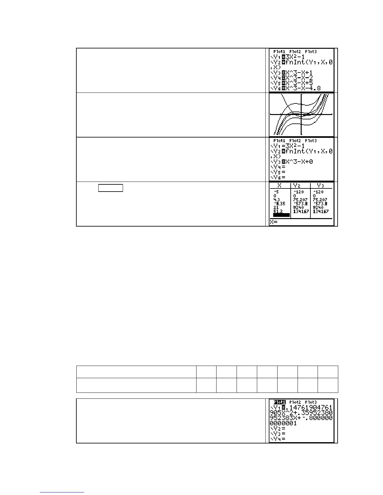
Enter f in Y1, fnInt(Y1, X, 0, X) in Y2, and F in Y3, Y4, Y5, and
Y6, using a different number for C in each function location.
(You can use the values of C shown to the right or different
values.)
Find a suitable viewing window and graph the functions Y1
through
Y6. The graph to the right was drawn with
−
3 ≤ x ≤ 3
and
−
20 ≤ y ≤ 20.
It appears that the only difference in the graphs of Y2 through Y6
is the y-axis intercept. But, isn’t C the y-axis intercept of each of
these antiderivative graphs?
Clear
Y4, Y5, and Y6. Turn off Y1 and change the 1 in Y3 to 0.
Press GRAPH and draw the graphs of Y2 and Y3. You should
see only one graph.
Set the calculator
TABLE to ASK and enter some values for x. It
appears that
Y2 and Y3 are the same function.
CAUTION: The methods for checking derivative formulas that were discussed in Sections
4.3.2b and 4.3.2c are not valid for checking general antiderivative formulas. Why not? Because
to graph an antiderivative using
fnInt, you must arbitrarily choose values for the constant of
integration and for the input of the lower endpoint. However, for most of the rate-of-change
functions where f(0) = 0, the calculator’s numerical integrator values and your antiderivative
formula values should differ by the same constant at every input value where they are defined.
5.4 The Definite Integral
When using the numerical integrator on the home screen, enter fnInt(f(x), x, a, b) for a specific
function f with input x and specific values of a and b. (Remember that the input variable does
not have to be x when the function formula is entered on the home screen.) If you prefer, f can
be in the
Y= list and referred to as Y1 (or whatever location is chosen) when using fnInt.
EVALUATING A DEFINITE INTEGRAL ON THE HOME SCREEN We illustrate the
use of
fnInt with the function that models the rate of change of the average sea level. The rate-
of-change data are given in Table 6.18 of Example 3 in Section 5.4 of Calculus Concepts.
Time (thousands of years before the present)
−
7
−
6
−
5
−
4
−
3
−
2
−
1
Rate of change of average sea level
(meters/year)
3.8 2.6 1.0 0.1
−
0.6
−
0.9
−
1.0
Enter the time values in L1 and the rate of change of the average
sea level values in
L2. A scatter plot of the data indicates a
quadratic function. Find the function and paste it in
Y1.
(Draw the function on the scatter plot of the data to confirm that
it gives a good fit.)
Copyright © Houghton Mifflin Company. All rights reserved.
75

 Loading...


