TI-83, TI-83 Plus, TI-84 Plus Guide
strained optimization problem with the functions given in Example 1 of Section 10.3 – the
Cobb-Douglas production function
f(L, K) = 48.1L
0.6
K
0.4
subject to the constraint g(L, K) =
8L + K = 98 where L worker hours (in thousands) and $K thousand capital investment are for a
mattress manufacturing process.
We first find the critical point(s). Because this function does not yield a linear system of
partial derivative equations, we use the algebraic method. We employ a slightly different order
of solution than that shown in the text. The system of partial derivative equations is
28.86
L
−
0.4
K
0.4
= 8λ
19.24L
0.6
K
−
0.6
= λ
8L + K = 98
⇒ 28.86L
−
0.4
K
0.4
= 8(19.24L
0.6
K
−
0.6
)
[4]
[5]
⇒
= 98 – 8L
Equation 4 was derived by substituting λ from the second equation on the left into the first,
and equation 5 was derived by solving the third equation on the left for
K. We now solve this
system of 2 equations (equations 4 and 5) in 2 unknowns (
L and K) using the methods shown
on page 106.
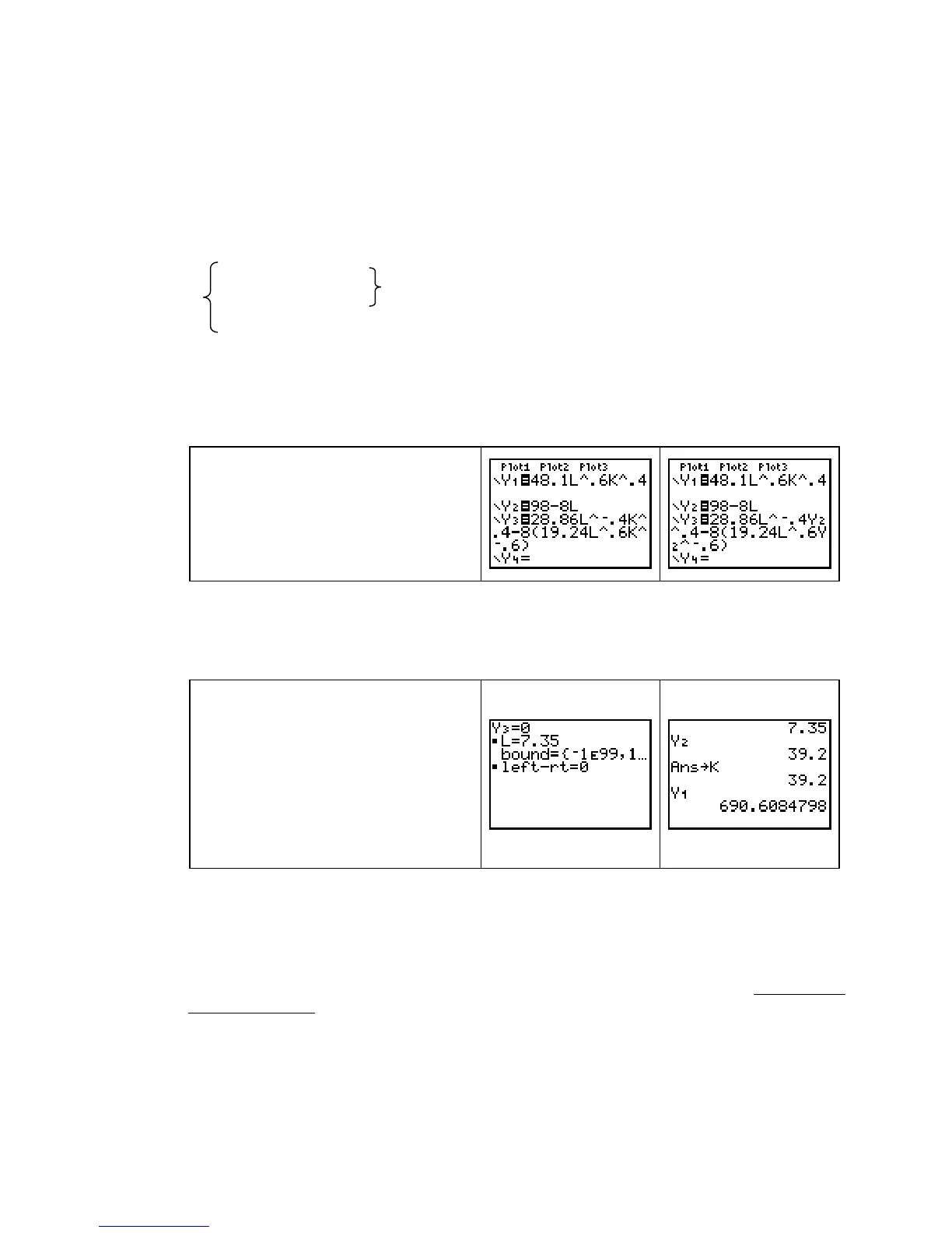
Clear the
Y= list. Enter the function f
in
Y1 and the expression for K in Y2.
Rewrite the other equation (equation 4)
so that it equals 0, and enter the non-
zero side in
Y3. Substitute Y2 into Y3.
(See the note below.)
NOTE: Remember that K = Y2. Put the cursor on the first K in Y3 and replace K by Y2.
Do the same for the other
K in Y3. The expression now in Y3 is the left-hand side of an
equation that equals 0 and contains only one variable, namely
L. (We are not sure how
many answers there are to this equation.)
Use the SOLVER to solve the equation
Y3 = 0. Try several different guesses
and see that they all result in the same
solution.
The calculator stores the value of
L.
Now return to the home screen and
evaluate Y2. Store this value in K.
Enter
Y1 to display the value of f at this
point.
Classifying critical points when a constraint is involved is done by graphing the constraint
on a contour graph or by examining close points. Your calculator cannot help with the contour
graph classification – it must be done by hand. We illustrate the procedure used to examine
close points for this Cobb-Douglas production function
.
We now test close points to see if this output value of
f is maximum or minimum. Remem-
ber that whatever close points you choose, they must be near the critical point and
they must be
on the constraint g.
WARNING: Do not round during this procedure. Rounding of intermediate calculations
and/or inputs can give a false result when the close point is very near to the optimal point.
Copyright © Houghton Mifflin Company. All rights reserved.
111

 Loading...


