To analyze a transient signal with time gating
This procedure assumes that the steps in “To set up transient analysis”
have been performed. If not, do so before continuing.
1. Turn on time gating, set the gate length, and set up the knob to move the gate:
Press [
Time
], [gate on ], [gate length], 3, [
us
], [
ch1 gate dly
].
Press the [
Marker|Entry
] hardkey so that the knob’s “Entry” LED is on.
2. Rotate the knob to move the gate over the very first part of the transient signal
appearing in the lower trace; see the plot below.
3. Set up the marker to show the movement of the spectrum’s peak:
Press [
A
], [
Marker Function
], [
peak track
on
].
Press [
Shift
], [
Marker⇒] (turns offset marker on and zeros it).
4. Now, move the time gate across the transient signal’s time display (by turning
the knob) and note the movement of the spectrum peak:
Press [
Time
], and make sure [
ch1 gate dly
] is selected (if not, press it).
Press [
Marker|Entry
] if the knob’s “Entry” LED is not on.
Rotate the knob, moving the gate further to the right into the transient
signal and stop long enough for the spectrum to update. Then move it
again and stop. The reference marker (square) remains at the location of
the “transient start up” making it easier to see the carrier movement as
the regular marker (diamond) tracks the peak. Marker readouts in the
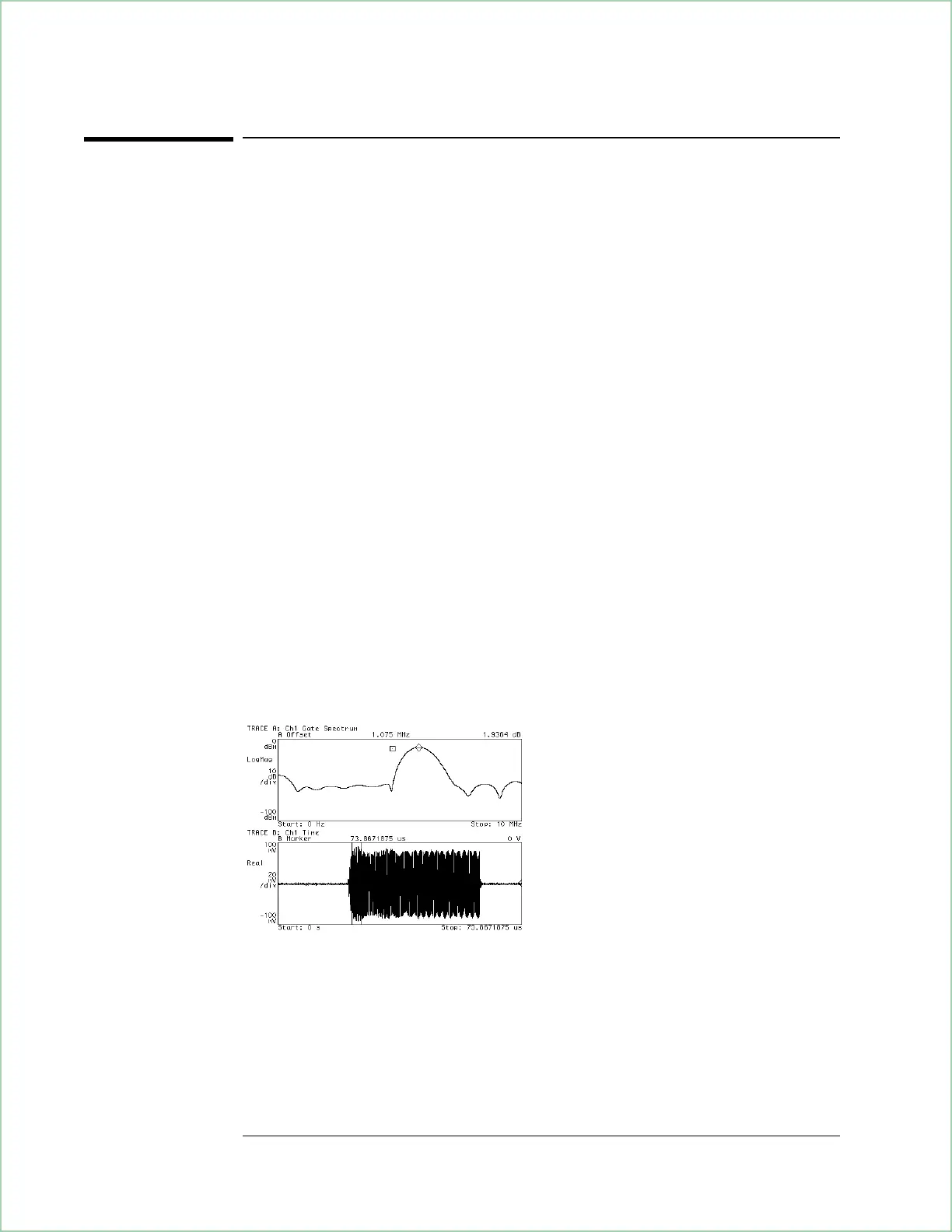
display pictured below show that early in the transient there is as much
as 1.00 MHz variation in carrier frequency.
With time gating on, the spectrum shown (top) is that of the data inside
the gate markers (bottom). In this case, moving the time gate across the
time signal (bottom) shows that the carrier frequency varies with time
(the spectral peak moves). We can use FM demod to show this, too.
(grids were turned off in the illustration to highlight the gate markers.)
Characterizing a Transient Signal
3-4