5. Set the number of frequency points for your signal. The number of frequency
points must be greater than the number of samples in a segment divided by
2.56 (real) or 1.28 (complex):
For 10 segments of 1920 samples:
1920 samples
1.28
= 1500 −−> Use 1601 freq. pts.
For 12 segments of 1600 samples:
1600 samples
1.28
= 1250 −−> Use 1601 freq. pts.
For 20 segments of 960 samples:
960 samples
1.28
= 750 −−> Use 801 freq. pts.
For this example, use 801 frequency points:
Press [
ResBW/Window
], [num freq points], 801.
6. Set the frequency span to obtain the desired sample frequency. For real
signals, divide the sample frequency by 2.56; for complex signals, divide by 1.28:
Frequency span (complex)=
3.84 MHz
1.28
= 3 MHz
Press [
Frequency
], [span], 3, [MHz].
7. Set the time-record length equal to the length of one segment:
Length of one segment =
960 samples
3.84 MHz
= 250 µ sec
Press [Time], [main length], 250 [µ s].
8. You are now ready to create a contiguous waterfall or spectrogram display for
your computer-generated data. Take note of the number of segments (time
records) needed for the waterfall or spectrogram display (from step 5) and see
‘’To create a long waveform using ASCII data’’ for further instructions.
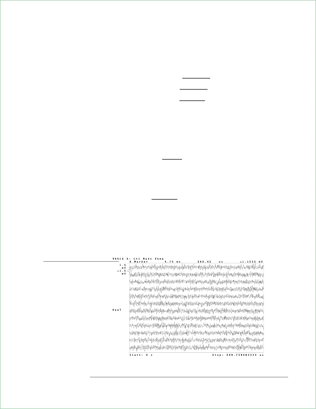
Here is a contiguous waterfall display
created using the parameters from
this procedure. The overall length is
250 µs and the marker shows
∆tat
260.42 ns. You add ∆t to the stop time
to determine the length of each trace.
You then multiply the length of each trace
by the total number of traces to compute
the length of the waterfall display.
You may notice that the stop time is not
250
µs. The stop time does not include
∆t for the last point.
Creating Arbitrary Waveforms
6-13
 Loading...