90 | PGC5000 GEN 2 | 892 J006 MNAH
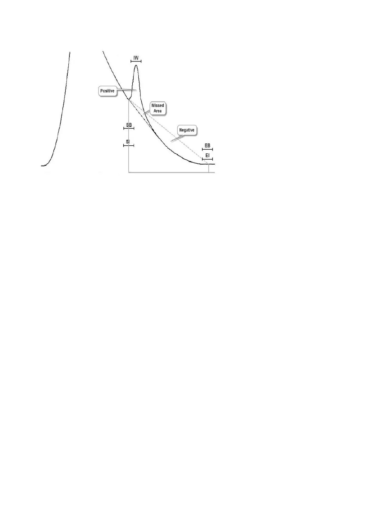
Figure 5-7: Baseline correction, tangent skim
5.4 Component detection (EZ peak)
The analyzer currently uses min-max peak detection as described in this section. For PGC5000
V3.0.2.1 and later, and for PGC5000 Generation 2, an EZ Peak feature is included in the software. It
allows users to define a peak area by entering only two variables: Component Retention Time (RT)
and a Threshold measurement.
EZ Peak requires two sequence Time-Coded Functions (TCF), Threshold and Component RT:
⎯ The Threshold TCF provides the noise multiplier used to compute the noise threshold. This TCF
appears only once and must precede any Component RT TCF. It must be placed in a quiet
zone of the signal at least two seconds after an Autozero. At the time specified in the TCF, the
threshold is computed from the previous 100 samples.
⎯ The Component RT TCF defines an expected retention time and a window encompassing that
time within which a peak is expected. It provides the bounds for the crest only and needs to
be wide enough to catch the crest. If there are multiple peaks within the window, the
algorithm selects the one closest to the user-defined retention time.
5.4.1 EZ peak calculations
Most chromatographic peaks take on the general form of a classical Gaussian curve and are analyzed
mathematically. The graph of a Gaussian curve is a characteristic symmetrical bell curve shape that
quickly falls off toward plus/minus infinity. EZ Peak detection utilizes a second derivative algorithm to
detect the presence of a peak. Derivatives enhance the ability to isolate regions in which peaks occur
by allowing the algorithm to search for a change in sign.
While it is visually obvious, locating a peak is not a simple task for a computer. Signal noise
complicates the decision of when peaks, valleys, and return to baseline occur. The user sets up five
separate windows for each peak: start of baseline, start of integration, crest, end of integration, and
end of baseline.
The second derivative measures how the rate of change of a quantity is itself changing and is set
using a threshold value. At the curve’s flex point on the leading side of the peak, the second
derivative crosses from positive to negative, and at the flex point on the trailing side, the derivative
crosses from negative to positive. Between those points a single peak will be found. A curve with
multiple crests has two sets of crossover points.
An advantage of the second derivative approach is shoulder detection (i.e., a bump on the side of a
large peak, caused by an underlying small peak, too small to form a valley between the two crests).
5.4.2 Identify peaks
At some point, the signal emerges above the noise enough to signify a peak has started. The second
derivative does not solve the problem of knowing when the peak actually starts, but it gives a starting
position to watch.
The second derivative algorithm measures the noise as a standard deviation in a quiet range of the
signal over a one second period (100 samples). The second derivative algorithm requires a minimum
of ten consecutive samples above the threshold before it is deemed a peak. As some noise may still