Section 1 - Introduction
1-3
The program works in the following manner:
1.
Load preliminary scan and obtain regions of interest from operator.
2.
Estimate k as an average value of:
k = [L
tissue
- L
air
] / [H
tissue
- H
air
]
where L
tissue
indicates a low-energy measurement with tissue-equivalent material
interposed by the filter drum, and L
air
, H
tissue
and H
air
are similarly defined.
Note:
The subscript "
air
" designates the filter drum segment that is empty (i.e., contains neither
bone- nor tissue-equivalent material).
3.
Using this value of k, calculate Q for each point scanned using the formula given above
(Q = L - kH). This array of Q values constitutes a "Q scan". Displays the Q scan.
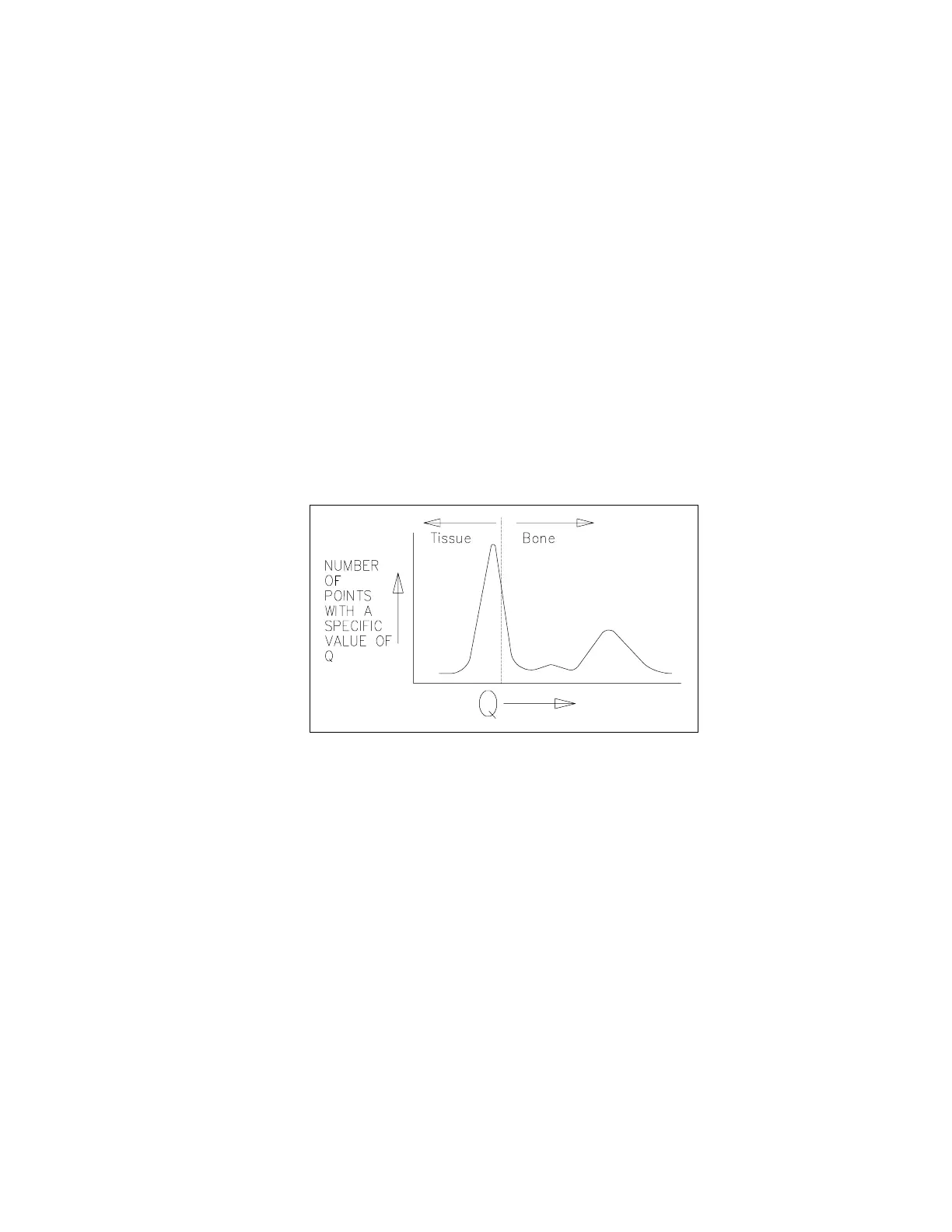
4.
Compile a histogram of the Q values. Because a large portion of the scan contains soft
tissue only, this histogram will have a large peak. Choose a threshold value just above
this peak, and apply that value to discriminate, point by point in the Q scan, between
"bone" points (whose Q is above the threshold) and "non-bone" points (whose Q is
below the threshold).
Figure 1-2. Q Scan Plot
5. Use the "non-bone" points to calculate a baseline value for each scan line. Using these
points, form a new histogram and repeat steps 4 and 5 until the results converge.
6. Smooth the segment boundaries to eliminate isolated noise-generated "bone" points.
7. Display the "bone" and "non-bone" points for operator approval.
8. Determine the constant of proportionality (d
0
) that relates the Q values to actual BMC
(grams). That constant is determined by measuring how much Q shifts when bone-
equivalent material is interposed by the filter drum.
9. Calculate the total bone mineral values by adding up the Q values for all "bone" points
in each region of interest (e.g., each vertebra), and multiplying by d
0
.
10. Determine the bone areas by counting the number of "bone" points in each region of
interest.
11. Calculate bone mineral density as: