Library of Function Blocks
4.21
The points of the adaptative gain curve are given as percentage of the selected variable on the axis
of the abscissa X and by the gain G on the axis of ordinate Y. The gain modifies the tuned
constants: K
P
, T
R
and T
D
into K
P
' , T
R
' and T
D
' as follows:
KpG Kp' ⋅=
G
T
Tp
R
='
DD T G 'T ⋅=
Gain G may affect the PID, PI, P, I and D actions. Selection is performed by parameter CAAD which
also inhibits Adaptative Gain action when CAAD=0. The adaptative gain is recommended for highly
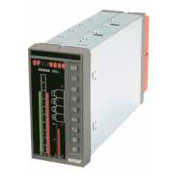
nonlinear controls. A classic example of adaptative gain is the drum level control of a boiler.
LIC
LT
WATER
TEAM
Fig 4.9.5 - Simple Drum Level Control of a Boiler
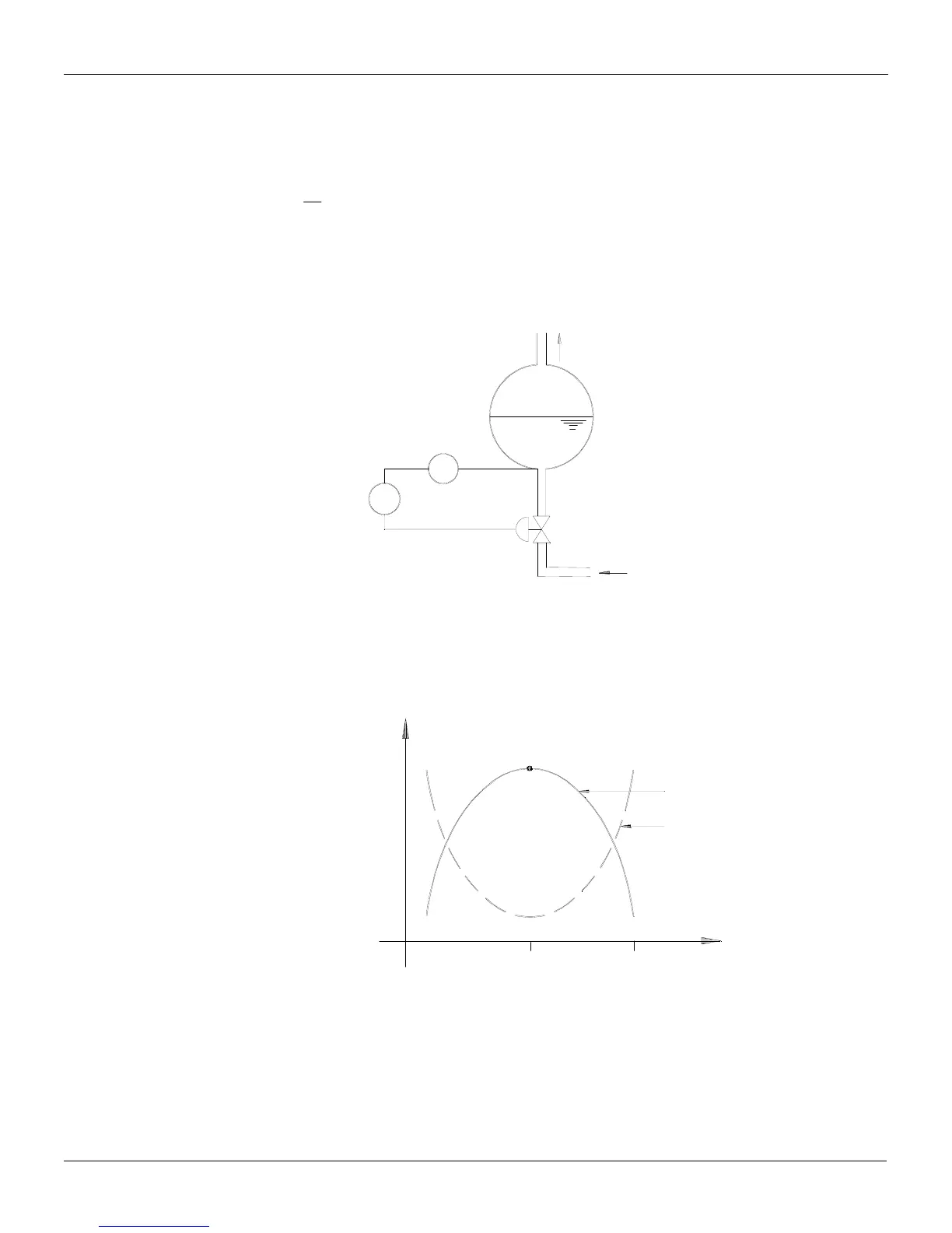
The volume variations are nonlinear with the level variations. The dotted line of Figure 4.9.6 show
the volume gain with the level. Note that the volume varies slowly (low gain), around 50% level and
varies very fast (high gain) around the level extremes. The control action must have a gain that is
the inverse of the process gain. This is shown by the continuous line of Fig 4.9.6.
AIN
CONTROLLER
GAIN
PROCESS
GAIN
100%
50%
0
LEVEL
Fig 4.9.6 - Process and Controller Gain
The adaptative gain characteristic can be configured as shown in Fig 4.9.7. This curve can be
represented by the following points of Curve 1: (X1 = 0; Y1 = 0.2; X2 = 20; Y2 = 0.8; X3 = 40; Y3 =
.96; etc.). 0