The reason this is such an interesting (and thus preferred) representation for the CDF and EDF is
that on this scale the CDF of a Gaussian PDF is a straight line. When the CDF or EDF is o
modified symmetric form, then their graphs appear as the upper lines of a triangle. Below is a plot
of an EDF (simulation) for a Gaussian PDF with
f the
a sigma of 1 picosecond.
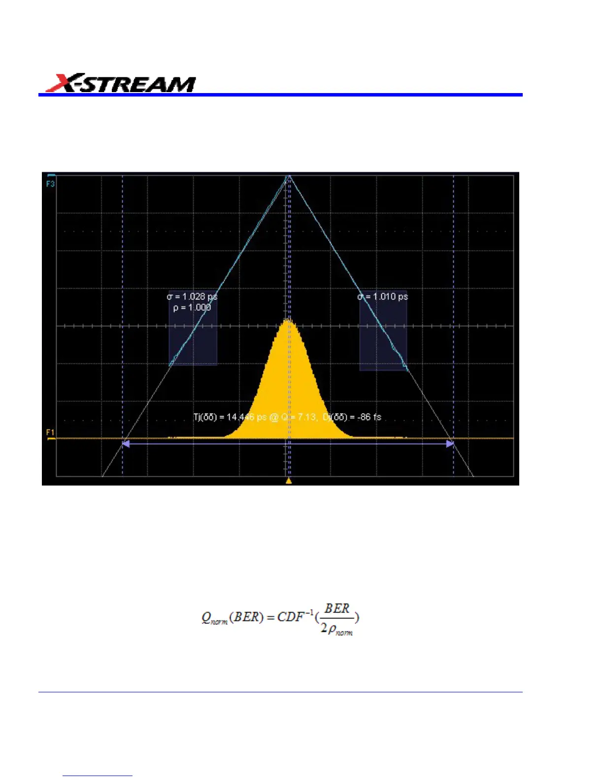
The other interesting attribute of this representation is that the slope of the lines give the sigma of
the distribution. This is all common treatment so r. All is well for a single Gaussian distribution.
Now, enter the idea that this coordinate transformation should have a variable normalization
s normalization is such that when the area of an un-normalized Gaussian is ρ
norm
, then
=0,
fa
factor. Thi
that resulting CDF manifests as straight lines with slope revealing sigma, and intercept with Q
giving the mean of the Gaussian PDF. This is the “normalized Q-Scale” where:
As an example, when two different Gaussian distributions are analyzed in this way, their EDFs
appear as below. The linear fits on this coordinate scale yields the proper (simulated) values for
their sigmas and means.
392 SDA-OM-E Rev H