SDA Operator’s Manual
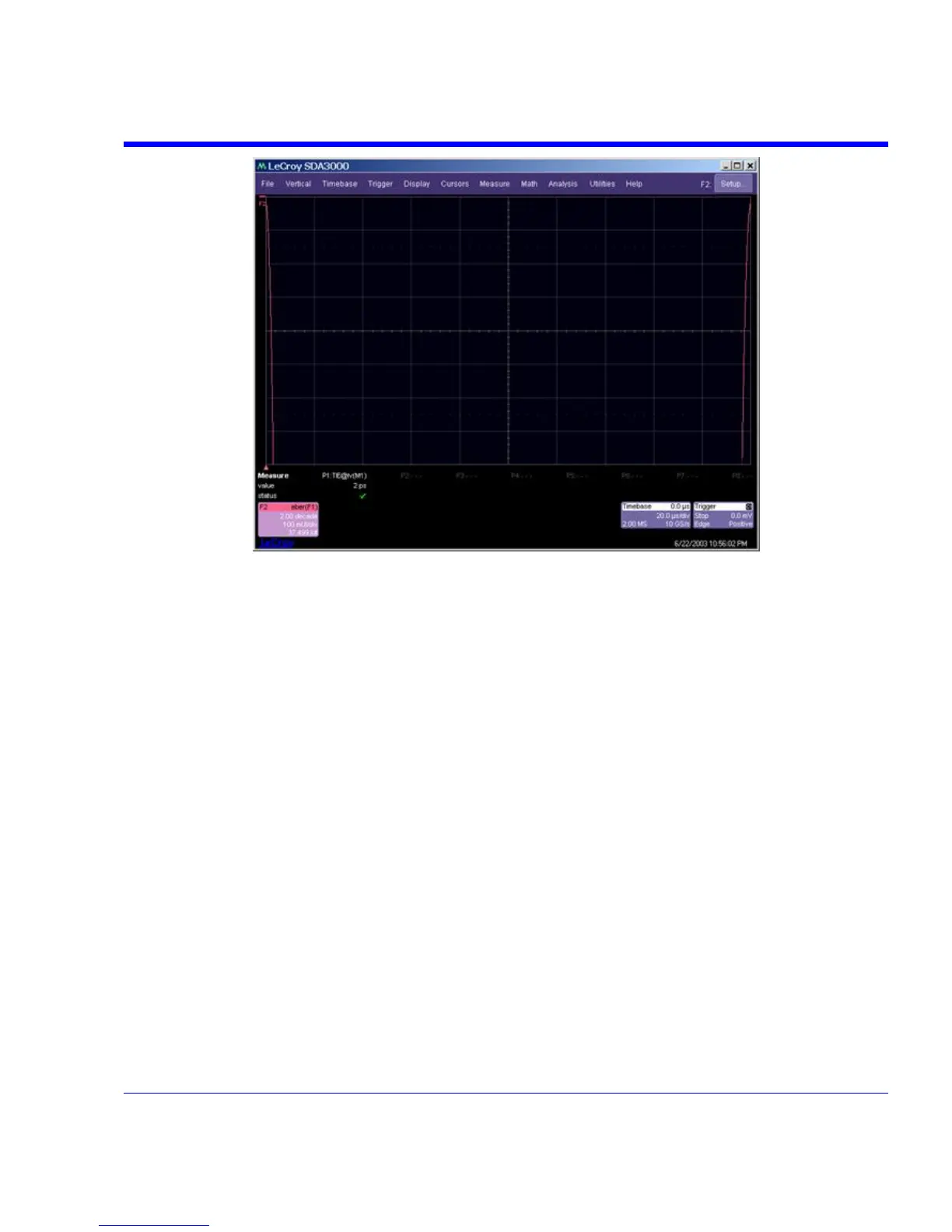
Figure 10. The bathtub curve is constructed by rescaling the total jitter curve in Figure 9 to one unit
interval, and centering the right side of the total jitter curve at 0 UI and the left side at 1 UI (the left
and right sides of the bathtub curve).
A common way to view the total jitter is by plotting the bit error rate as a function of sampling
position within a bit interval. This curve, commonly referred to as the “bathtub” curve is derived
from the total jitter curve by scaling it to one bit interval (UI). The right half of the bathtub curve is
taken from the left half of the total jitter curve and the left half is taken from the right half of the
total jitter curve. The bathtub curve corresponding to the total jitter curve in Figure 9 is shown in
Figure 10.
Extrapolating the PDF
Measuring the total jitter requires that the probability density function (PDF) of the jitter be known
exactly. The SDA measures the jitter PDF by collecting a histogram of TIE measurements. This
histogram approximates the PDF by counting the number of edges occurring within the time
period delimited by each bin in the histogram. In order to accurately measure jitter contributions at
very low bit error rates such as 1012, the histogram must contain measurements with populations
that are below 1 in 1016 (one TIE measurement out of 1016 at a certain value). This number of
data transitions would take approximately 38 days at 3 Gb/s. Measuring this number of edges is
clearly impractical.
SDA-OM-E Rev H 377