R&S ZVB - Page 56

R&S
®
ZVA / R&S
®
ZVB / R&S
®
ZVT System Overview
Screen Elements
Operating Manual 1145.1084.12 – 30 41
help system).
A comparison of the inverted Smith chart with the Smith chart and the polar diagram reveals many
similarities between the different representations. In fact the shape of a trace does not change at all if the
display format is switched from Polar to Inverted Smith or Smith – the analyzer simply replaces the
underlying grid and the default marker format.
Inverted Smith chart construction
The inverted Smith chart is point-symmetric to the Smith chart:
The basic properties of the inverted Smith chart follow from this construction:
 The central horizontal axis corresponds to zero susceptance (real admittance). The center of the
diagram represents Y/Y
0
= 1, where Y
0
is the reference admittance of the system (zero reflection).
At the left and right intersection points between the horizontal axis and the outer circle, the
admittance is infinity (short) and zero (open).
 The outer circle corresponds to zero conductance (purely imaginary admittance). Points outside
the outer circle indicate an active component.
 The upper and lower half of the diagram correspond to negative (inductive) and positive
(capacitive) susceptive components of the admittance, respectively.
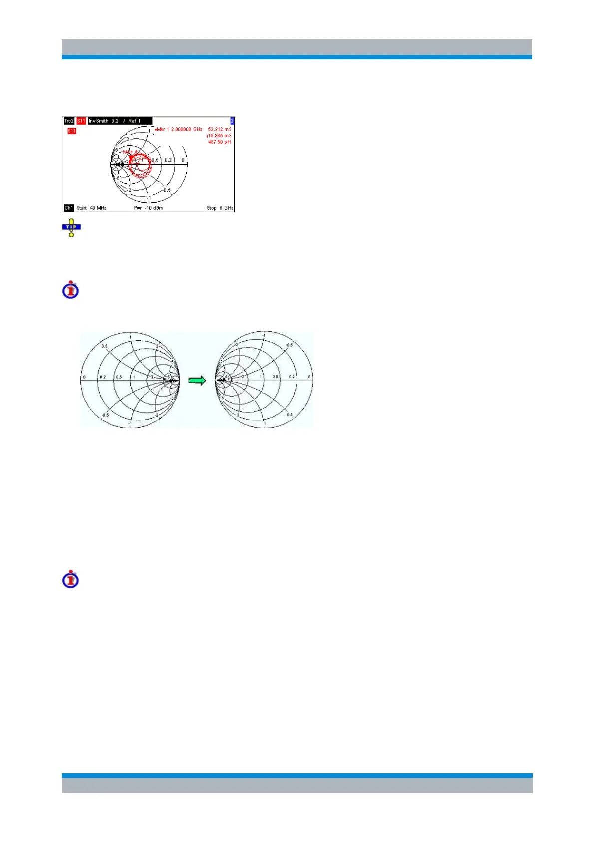
Example: Reflection coefficients in the inverted Smith chart
If the measured quantity is a complex reflection coefficient Γ (e.g. S
11
, S
22
), then the unit inverted Smith
chart can be used to read the normalized admittance of the DUT. The coordinates in the normalized
admittance plane and in the reflection coefficient plane are related as follows (see also: definition of
matched-circuit (converted) admittances):
Y / Y
0
= (1 - Γ) / (1 + Γ)
From this equation it is easy to relate the real and imaginary components of the complex admittance to the
real and imaginary parts of Γ