Creation of calibration curves
The illustrations below explain how the calibration curves are created. (
Learn about media family
calibration
on page 222)
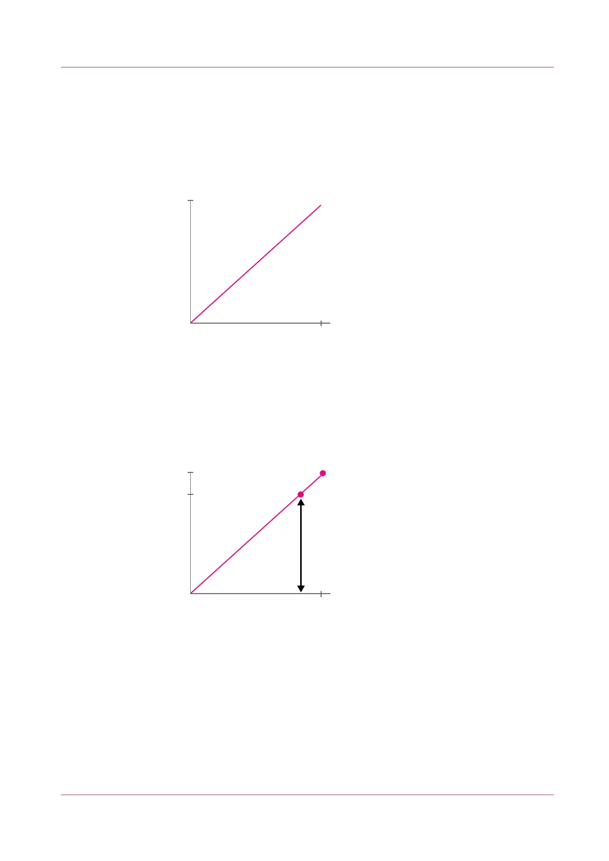
1. Imagine, you use an i1 spectrophotometer to measure a test chart with magenta gradients
from 0% to 100%. The measured Lab values will compose a straight line from white (Lab
0,0,0) to the Lab color value at 100%.
2. A Lab value is a three-dimensional value that does not allow for easy color comparisons. It
helps when a color value on this line could be expressed as a single value, such as the (ΔE)
metric to express a color difference.
A value based on a color difference can be created as follows. The difference between the Lab
value of a color and the Lab value of paper white (0,0,0) delivers a ΔE value. (
Learn about
color differences
on page 250)
The maximum color value (expressed in ΔE) refers to the 100% tone value.
3. When you perform a media family calibration, all measured values of the patches are
compared with the values expected from the output profile. PRISMAsync Print Server
calculates for every patch a correction value. The results are extrapolated to gradients that
have not been measured. In this example, patch 1 represents the 5% tone value and patch 5
the 100% tone value.
Creation of calibration curves
Chapter 15 - References
441