8.22
SEL-351A Relay Instruction Manual Date Code 20080213
Breaker Monitor and Metering
Demand Metering
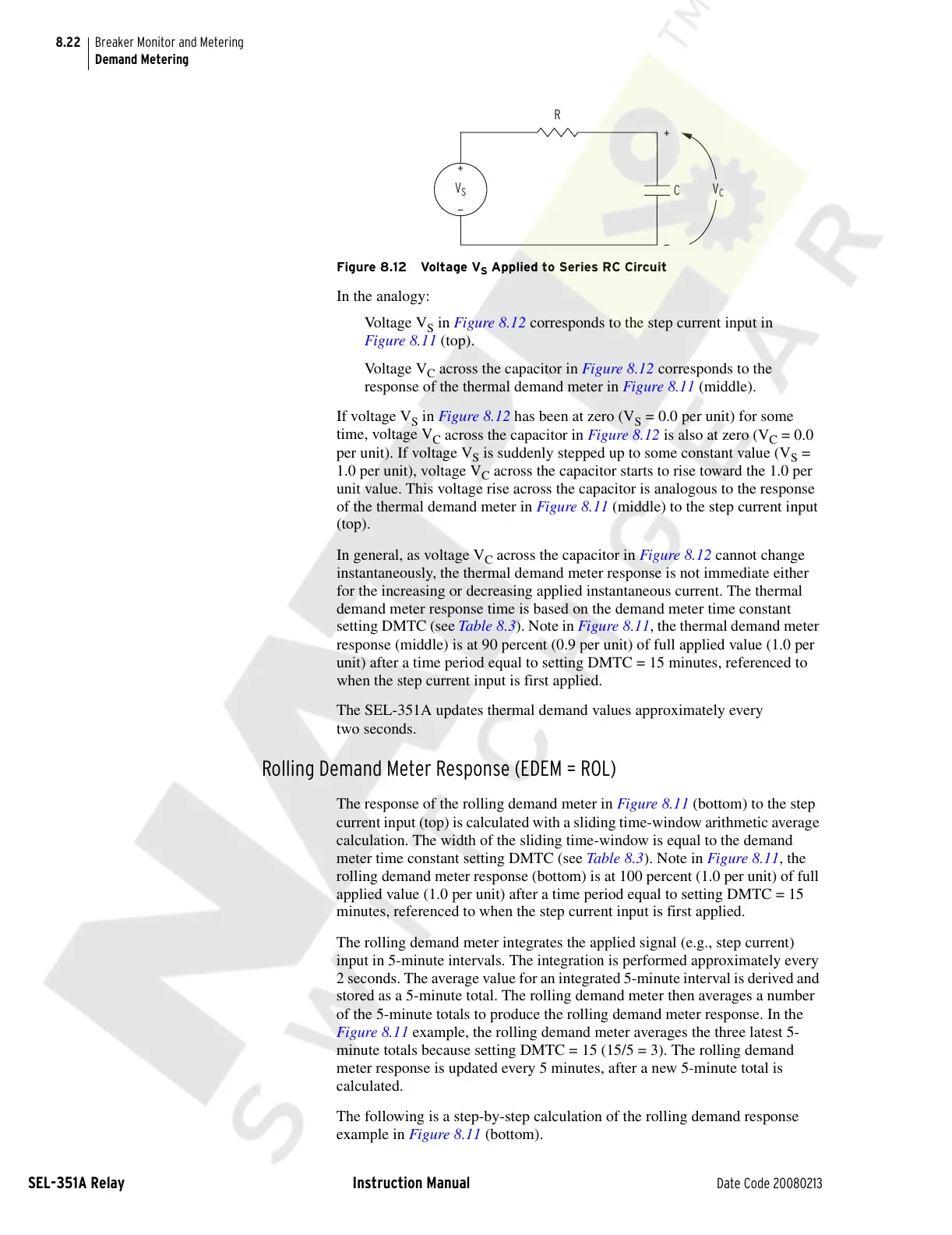
Figure 8.12 Voltage V
S
Applied to Series RC Circuit
In the analogy:
Voltage V
S
in Figure 8.12 corresponds to the step current input in
Figure 8.11 (top).
Voltage V
C
across the capacitor in Figure 8.12 corresponds to the
response of the thermal demand meter in Figure 8.11 (middle).
If voltage V
S
in Figure 8.12 has been at zero (V
S
= 0.0 per unit) for some
time, voltage V
C
across the capacitor in Figure 8.12 is also at zero (V
C
= 0.0
per unit). If voltage V
S
is suddenly stepped up to some constant value (V
S
=
1.0 per unit), voltage V
C
across the capacitor starts to rise toward the 1.0 per
unit value. This voltage rise across the capacitor is analogous to the response
of the thermal demand meter in Figure 8.11 (middle) to the step current input
(top).
In general, as voltage V
C
across the capacitor in Figure 8.12 cannot change
instantaneously, the thermal demand meter response is not immediate either
for the increasing or decreasing applied instantaneous current. The thermal
demand meter response time is based on the demand meter time constant
setting DMTC (see Table 8.3). Note in Figure 8.11, the thermal demand meter
response (middle) is at 90 percent (0.9 per unit) of full applied value (1.0 per
unit) after a time period equal to setting DMTC = 15 minutes, referenced to
when the step current input is first applied.
The SEL-351A updates thermal demand values approximately every
two seconds.
Rolling Demand Meter Response (EDEM = ROL)
The response of the rolling demand meter in Figure 8.11 (bottom) to the step
current input (top) is calculated with a sliding time-window arithmetic average
calculation. The width of the sliding time-window is equal to the demand
meter time constant setting DMTC (see Table 8.3). Note in Figure 8.11, the
rolling demand meter response (bottom) is at 100 percent (1.0 per unit) of full
applied value (1.0 per unit) after a time period equal to setting DMTC = 15
minutes, referenced to when the step current input is first applied.
The rolling demand meter integrates the applied signal (e.g., step current)
input in 5-minute intervals. The integration is performed approximately every
2 seconds. The average value for an integrated 5-minute interval is derived and
stored as a 5-minute total. The rolling demand meter then averages a number
of the 5-minute totals to produce the rolling demand meter response. In the
Figure 8.11 example, the rolling demand meter averages the three latest 5-
minute totals because setting DMTC = 15 (15/5 = 3). The rolling demand
meter response is updated every 5 minutes, after a new 5-minute total is
calculated.
The following is a step-by-step calculation of the rolling demand response
example in Figure 8.11 (bottom).
V
S
V
C
+
+
—
—
R
C
Courtesy of NationalSwitchgear.com
 Loading...