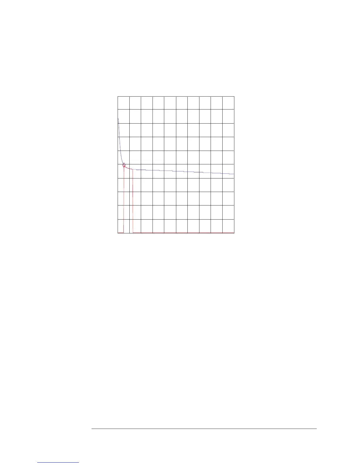
Figure 16-3.
Curve Fit with Restricted Fit Region Overlaid With a Synthesis
To make this easier to understand, consider the fit we used in this example. As
the order of the trial curve fit increased, the curve fit trace was too far away
from the synthesized trace to be considered a good fit. When the order reached
2 poles and 2 zeros, the curve fitter found a model whose frequency response
inside the fit region was sufficiently close to the synthesis trace to be
considered good. At this point, the analyzer used order reduction to try and
minimize the numerator order, but without success—in other words, given a
limited picture of the complete frequency response, the analyzer found an
alternative model that was sufficiently accurate over the fit region.
A comparison of the synthesis model and curve fit model over 51.2 kHz more
clearly shows the divergence between the two responses. This is shown in
figure 16-4. You can generate this display by changing the span to 51.2 kHz
and doing the synthesis with Trace A active. Then copy the curve fit table to
the synthesis table, change the synthesis register to D7, and do the synthesis
with Trace B active. Then change to the front/back display format. (If the pole
at 45 kHz and the zero at 65 kHz are not present, a curve fit over 1.28 kHz to
3.2 kHz will yield the original model, as shown in figure 16-5.)
0Hz 25.6kHz
A: D8Synthesis X:1.28 kHz Y:9.9128 dB
20
dB
0
dB
dBMag
2
dB
/div
X:1.28 kHz Y:9.91281dBB: D6CurveFit
20
dB
0
dB
dBMag
2
dB
/div
Scale Trace: A Ref Lvl: 0
Per Div: 2 Ref Pos: Bottom
Agilent 35607A
Curve Fit Option 1D3 Operator's Guide
16-20
 Loading...