Agilent Technologies 35670A

To measure a step response
The primary objective in designing a control system is to construct a system that
achieves the desired output level as fast as possible and maintains that output with
little or no variation or steady state error. The step response is a technique that
measures a control system’s compliance with the design goals. This task utilizes a
step signal created with the Arbitrary Source, Option 1D4.
1 Create and store a step signal in data register D1.
See “To create a step signal” in chapter 6.
2 Initialize the analyzer.
Press [
Preset
][
DO PRESET
].
Press [
Inst Mode
][
HISTOGRAM/TIME
].
Press [
Meas Data
].
Press [
CHANNEL 1 2 3 4
] to highlight 2.
Press [
UNFILTERD TIME CH2
].
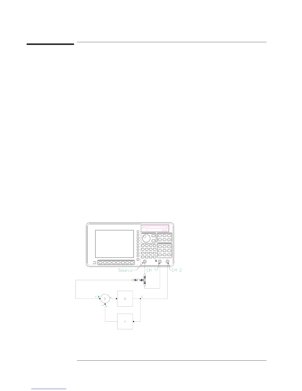
3 Connect the device-under-test (DUT) as shown in the illustration below.
4 Specify the measurement parameters.
Press [
Freq
][
RECORD TIME
] <number> <unit>.
Press [
Input
][
CH1 FIXED RANGE
] <number> <unit>.
Press [
Source
][
MORE CHOICES
][
ARBITRARY (D1 - D8)
].
Press [
Rtn
].
Press [
LEVEL
] <number> <unit>.
Press [
SOURCE ON OFF
] to highlight ON.
Agilent 35670A
Measuring Control Systems Operator's Guide
5-8