480 Graphs & Geometry
In this example, manipulating the intial term demonstrates that the
point of equilibrium in the rabbit and fox populations over the cycle
of 400 generations = (150, 50).
Graphing differential equations
You can study linear and non-linear differential equations and systems of
ordinary differential equations (ODEs), including logistic models and
Lotka-Volterra equations (predator-prey models). You can also plot slope
and direction fields with interactive implementations of Euler and
Runge-Kutta methods.
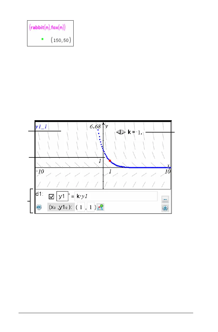
À Slope field
Á A solution curve passing through the intitial condition
 ODE editor:
– Checkbox for designating this ODE as active or inactive
–
y1 ODE identifier
– Expression
k·y1 defines the relation
– Fields (
1,1) for specifying initial condition
– Buttons for adding initial conditions and setting plot parameters
à Slider to control coefficient k of the ODE
Â
Á
À
Ã

 Loading...