prole and can be used for graphical editing of basic CAM
data points or advanced CAM nodes and segments.
Zoom in or zoom out is possible using the mouse wheel.
While zooming, the zoomed area is centered on the point
at which the mouse cursor is pointing. The maximum
possible horizontal zoom out is 360°. The vertical zoom is
not bounded. The horizontal zoom is always synchronized
with the velocity, acceleration, and jerk graph.
By pressing the center mouse button while dragging the
mouse, it is possible to move the center zoom point in
order to explore the graph while zoomed in. The visible
point area is between 0° and 360°.
The visual editing of CAM elements is performed by
selecting and dragging elements, or by using the available
context menus on the plot area. The visual editing of the
CAM elements varies across the dierent prole types and
element types (see chapter 5.7.7.6 Editing Basic CAM Proles
and chapter 5.7.7.7 Editing Advanced CAM Proles).
It is possible to select 1 or more CAM elements via 1 of
the following 2 methods:
•
Left-click on the desired element. Press the [Ctrl]
key on the keyboard and click on unselected or
selected elements to add or remove them from
the current selection.
•
Use the mouse to draw a box around the CAM
elements to select. To select an element, the box
must entirely encase the element. To add further
elements to the selection, press the [Ctrl] key on
the keyboard and draw another box encasing
those additional elements.
Velocity, acceleration, and jerk plot area
The velocity, acceleration, and jerk plot area is a 2-
dimensional plot of real numbers to show the 3 derivatives
of the rotor angle (vertical axis) in relation to the guide
value (horizontal axis). All 3 graphs are visualized in a
single plot area. The guide value axis is given in degrees
and the velocity, acceleration, and jerk graphs are given in
the units specied in the CAM Prole window toolbar. The
horizontal axis is labeled as Guide Value [degrees] and the
vertical axis is labelled as Value [unit], where Value denotes
the last activated graph (velocity, acceleration, or jerk) and
[unit] denotes the user-dened position unit for the graph.
The 3 graphs are rendered in the respective color specied
in the Options window. The default colors are:
•
Velocity: blue
•
Acceleration: green
•
Jerk: magenta
The mouse wheel and the center mouse button have the
same functionality as for the rotor angle plot area.
The plot area only visualizes the calculated velocity,
acceleration, and jerk graphs. No nodes or data points are
visualized in the plot area. It is not possible to select any
CAM elements on the graph.
5.7.7.6 Editing Basic CAM Proles
This section describes the specic visualization and editing
functionalities for basic CAM proles. Further information
about basic CAM can be found in chapter 2.4.5.4 Basic CAM.
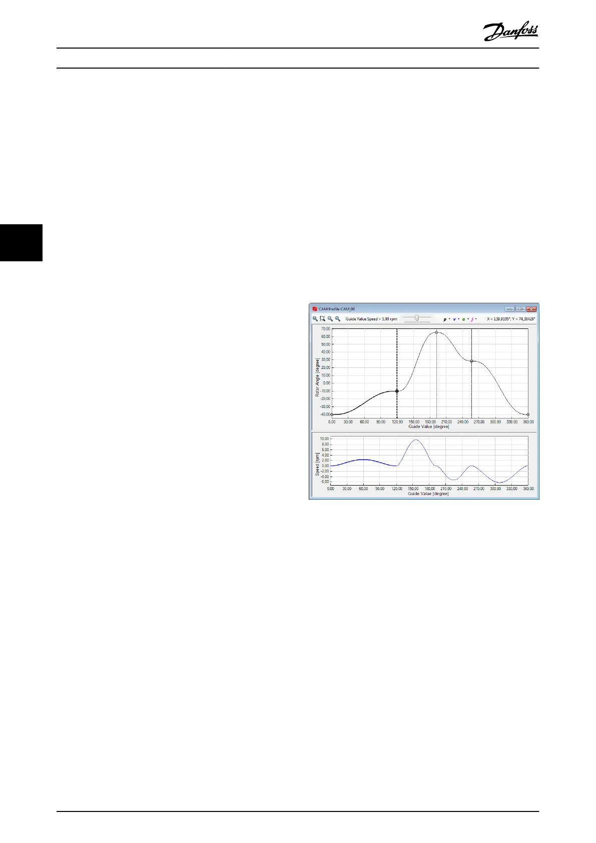
Data point and rotor movement visualization
When editing basic CAM proles, it is possible to place,
move, copy, and remove basic CAM data points from the
prole. The data points are visualized as circles in the rotor
angle plot area. Also, for every point, a dashed vertical line
is shown at its guide value position. It is possible to select
a data point by clicking on the respective circle or vertical
dash line that represents it.
Illustration 5.63 shows a CAM prole window for a basic
CAM with a selected basic CAM data point at the position
(120, -10) that can be moved in any direction.
Illustration 5.63 Editing a Basic CAM Prole
It is possible to graphically move a basic CAM data point
by dragging its circle. To move multiple basic CAM data
points at once, select multiple points and drag 1 of them:
the others are moved by the same oset as the dragged
point.
The resulting positions between the basic CAM data points
are visualized on the rotor angle plot area. Although the
resulting graphs look like segments, they cannot be
selected and are only updated after data point modi-
cations.
A data point is always connected with its 2 neighboring
data points, if existing. When moving a data point between
2 other data points, the graphs between the data points
are recalculated and reconnected.
Whenever the prole is not a full prole, it can be
visualized either as acyclic (prole starts with 1
st
data point
and ends at last data point) or as cyclic (last node is
virtually connected with rst node).
Operation with ISD Toolbox
VLT
®
Integrated Servo Drive ISD
®
510 System
144 Danfoss A/S © 01/2017 All rights reserved. MG36D102
55
 Loading...