RTC6 boards
Doc. Rev. 1.0.21 en-US
7 Basic Functions for Scan Head Control and Laser Control
205
• The percent value is relative to the 100% value
from set_auto_laser_control (Parameter
Value
)
or dynamically from a ““vector-controlled laser
control””, see Section ”Vector-Defined Laser
Control”, page 206.
In the following example, a nonlinearity factor of
1.2 is set for a 1.5x multiple of the target value:
Percent<n> = 150
Scale<n> = 1.2
• For
<Value>
, the following ranges apply
0.0 Percent 400.0 and
0.0 Scale(Percent) 4.0.
• Each instruction must be in a separate line.
• Spaces and tabs in a line (for example, between
’
=
’ and
<Value>
) are ignored.
• Empty lines are ignored.
• Data points with invalid values are ignored.
• The data point of a particular index
<n>
is ignored
if the corresponding
Percent<n>
and/or
Scale<n>
definition is missing.
• The semicolon ’;’ can be used for comments. All
characters in a line following a semicolon are
ignored.
• The instructions for data points in the table can
be ordered as desired.
• Indices for data point pairs in the table can be
selected as desired within the range [1…50] (the
table is then automatically sorted by ascending
percent values).
• If the table contains no valid data point, then
load_auto_laser_control has no effect
(return value 1 or 13).
• If there is no entry for Percent = 0.0, then an
entry with
Scale
= Min(
Scale<i>
) is inserted (the
smallest allowed value defined in the table is used
for lower percent values). Likewise for
Percent = 400.0 with Max(
Scale<i>
).
After load_program_file this function is initialized
for all percentage values with “Factor 1.0”, the
nonlinear laser control is “deactivated”. Alternatively,
this can also be achieved with
Name
= NULL in
load_auto_laser_control.
The table can be saved by create_dat_file.
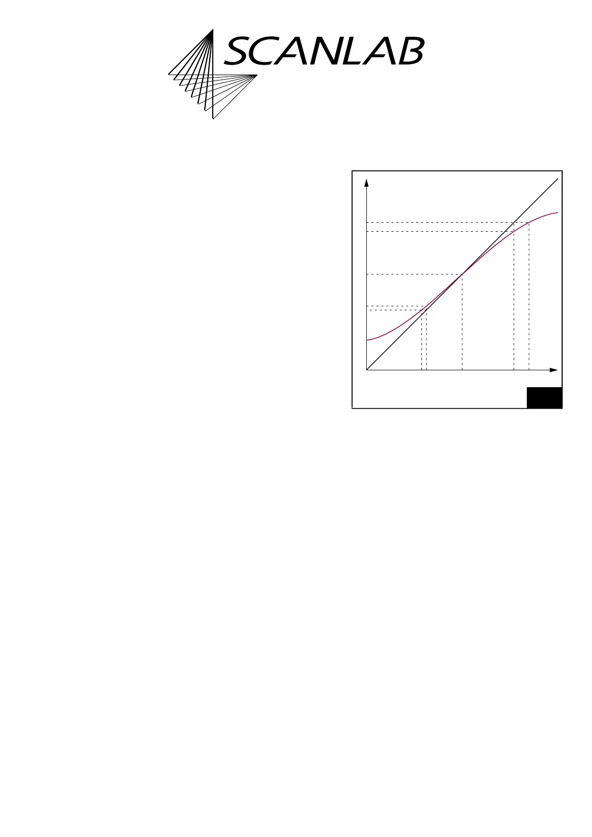
The example diagram in Figure 59 illustrates how the
nonlinearity curve can be determined.
The straight line in the diagram describes an ideal
relationship between laser power and the laser
control signal parameter (here, the term laser power
also represents the pulse
frequency = 0.5/
LaserHalfPeriod
), the curved line
simulates a realistic relationship.
S
0
is the signal parameter value defined as the target
value and P
0
is the associated laser power. At point
(S
0
P
0
) (this corresponds to the data point
Percent0
= 100,
Scale0
= 1.0) the two curves are
normalized to each other. The combination of a
nonlinearity curve with a ““vector-controlled laser
control”” is therefore generally not recommended.
An increase (decrease) of the signal parameter to S
1
(S
2
) results in an ideal laser power P
1
(P
2
) and a real
laser power P
1r
(P
2r
). For the actually desired laser
power P
1
(P
2
), a corrective signal parameter value S
1k
(S
2k
) is needed. The following two value pairs are
then to be entered as data points for the nonlinearity
curve:
Percent1
= S
1
/S
0
× 100 = P
1
/P
0
× 100
Scale1
= S
1k
/S
1
Percent2
= S
2
/S
0
× 100 = P
2
/P
0
× 100
Scale2
= S
2k
/S
2
59
Laser power progression – example of determining a
nonlinearity curve.
Signal
S
0
S
1
S
1k
S
2
S
2k
0
P
0
P
1
P
1r
P
2
P
2r
Real
curve
Ideal
curve
Laser
power